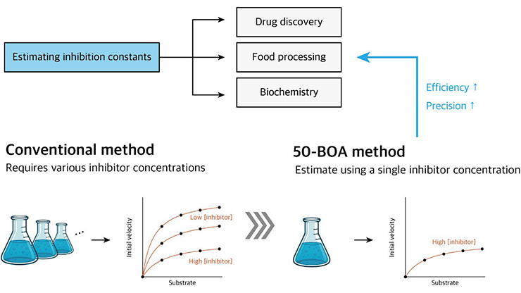
A Model-informed Shortcut to Estimate Inhibition Constants

Inhibition constants are fundamental parameters that quantify drug-drug interactions and guide medication dosing. Conventional estimation methods—currently used in more than 60,000 studies—require extensive experimental data from varied conditions to estimate these constants. We developed a novel approach that substantially reduces the necessary experimental requirements for estimation while preserving, and even sometimes improving, accuracy and precision relative to standard techniques. 

The Problem With Conventional Estimation

When a patient takes two drugs simultaneously, one drug (inhibitor) may bind to the target enzyme of another drug (substrate) and interfere with the substrate’s metabolic process (see Figure 1). This phenomenon—known as enzyme inhibition—plays a critical role in clinical pharmacology, as it can lead to increased dosage levels, reduced efficacy, or heightened toxicity of the affected drug [3]. Given inhibitor concentration \(I_T\), the initial metabolic velocity (\(V_0\)) of a substrate with initial concentration \(S_T\) decreases by following the subsequent inhibition model \((1)\):

\[V_0:=\frac{dP}{dt}\Bigg |_{t=0}=\frac{V_\textrm{max}S_T}{K_M(1+\frac{I_T}{K_{ic}})+S_T(1+\frac{I_T}{K_{iu}})}. \tag1\]

Here, \(V_\textrm{max}\) and \(K_M\) are parameters that pertain to the substrate and are usually known in advance from \(I_T=0\) data. \(V_\textrm{max}\) is a maximal metabolic velocity and \(K_M\) is a substrate concentration that reaches half of \(V_\textrm{max}\). Additionally, \(K_{ic}\) and \(K_{iu}\) are the inhibition constants, which respectively serve as dissociation constants of the inhibitor to the enzyme and enzyme-substrate complex (see Figure 2). They not only represent the potency of inhibition but also allow us to infer the mechanism of inhibitors or influence drug dose adjustments. If \(K_{ic}<K_{iu},\) for instance, dose adjustments can help avoid clinical risks; however, doing so is challenging when \(K_{iu}<K_{ic}.\) The precise and accurate estimation of these parameters is therefore critical [3, 8]. 

Conventionally, scientists estimate inhibition constants by first determining the half maximal inhibitory concentration (\(\textrm{IC}_{50}\)),¹ then fitting \((1)\) to initial velocity data from various combinations of \(S_T\) and \(I_T\) around \(\textrm{IC}_{50}\) (see Figure 3) [2]. Although this method has been the standard for decades, its optimality and sufficiency for precise estimation remain unproven. In fact, multiple studies have observed inconsistencies in reported inhibition constants [7, 9]. 

A Model-guided Approach

To address the aforementioned issues with conventional estimation methods, we conducted error landscape and sensitivity analyses across various experimental conditions [6]. Our results indicate that data obtained via a single inhibitor concentration \(I_T\) that is greater than both inhibition constants is sufficient for precise estimation (see Figure 4b). In contrast, estimation is highly sensitive to measurement errors when we collect data at \(I_T\) values that are below both inhibition constants (see Figure 4a). These findings suggest that the conventional approach may collect unnecessary or even detrimental data, which can reduce estimation accuracy and precision. But since the true values of the inhibition constants are not known a priori, it is difficult to identify the experimental data in advance that are informative, redundant, or potentially harmful.

IC₅₀ as a Guide

To identify informative experimental data without prior knowledge of the inhibition constants, we focused on \(\textrm{IC}_{50}\) — which scientists typically disregard after initial experimental setup (see Figure 3). \(\textrm{IC}_{50}\) satisfies the well-known weighted harmonic mean relationship with the inhibition constants [5]:

\[\frac{1}{\textrm{IC}_{50}}=\frac{\alpha}{K_{ic}}+\frac{1-\alpha}{K_{iu}}=:\frac{1}{H(K_{ic},K_{iu})}, \qquad \alpha=\frac{K_M}{S_T+K_M}. \tag2\]

This relationship implies that choosing \(I_T\ge\textrm{IC}_{50}\) ensures that either \(I_T\ge K_{ic}\) or \(I_T \ge K_{iu},\) providing a practical criterion for the collection of only informative data while avoiding the bias and sensitivity issues that arise when \(I_T\le\min\{K_{ic},K_{iu}\}.\) We incorporated this relationship into our estimation process as an \({IC}_{50}\)-based regularization term in \((3)\): 

\[\textrm{Total error}=\textrm{fitting error}+\lambda \times \Bigg(\frac{\textrm{IC}_{50}-H(K_{ic},K_{iu})}{\textrm{IC}_{50}}\Bigg)^2. \tag3\]

Here, we use the mean of the squared relative error between \(V_0\) data and \((1)\) to calculate fitting error. \(\textrm{IC}_{50}\) is an observed value, \(H(K_{ic},K_{iu})\) is a computed \(\textrm{IC}_{50}\) via \((2)\), and \(\lambda\) is a regularization constant that is obtained with cross-validation. 

This approach enables precise, accurate estimation of the inhibition constants by using data from a single \(I_T \ge \textrm{IC}_{50},\) even when \(I_T\) is less than both constants (see Figure 5). We combine these strategies and propose the \(IC_{\textit{50}}\)-based optimal approach (50-BOA) for efficient estimation of inhibition constants (see Figure 1).

Validating 50-BOA: Accurate and Efficient Estimation With Real Data

Applying 50-BOA to experimental data achieves an accuracy level that is comparable to the conventional approach (see Figures 6a and 6b). Additionally, the 95 percent confidence intervals are similar to or narrower than those from the conventional method. As a result, 50-BOA allows for equal or improved accuracy and precision while reducing the required experimental data by more than 75 percent (see Figure 6c).

We expect our study to enhance the efficiency of enzyme inhibition evaluation in both drug development and other relevant fields like the food industry, which utilizes enzyme inhibition to prevent food browning and spoilage [1]. Moreover, we anticipate that our work will catalyze future research into optimal, experimentally-feasible designs — ultimately extending beyond enzyme inhibition to various biological systems.

¹ Half maximal inhibitory concentration (\(\textrm{IC}_{50}\)) is an inhibitor concentration where the effect of inhibition compared to \(I_T=0\) reaches 50 percent.

Acknowledgments: We would like to acknowledge the coauthors of this study: Sang Kyum Kim, Hwi-yeol Yun, and Jang Su Jeon of Chungnam National University.

References
[1] Ackaah‐Gyasi, N.A., Zhang, Y., & Simpson, B.K. (2016). Enzymes inhibitors: Food and non‐food impacts. In R. Rai V. (Ed.), Advances in food biology (pp. 191-206). Hoboken, NJ: Wiley.
[2] Copeland, R.A. (2013). Evaluation of enzyme inhibitors in drug discovery: A guide for medicinal chemists and pharmacologists. Hoboken, NJ: John Wiley & Sons.
[3] Deodhar, M., Al Rihani, S.B., Arwood, M.J., Darakjian, L., Dow, P., Turgeon, J., & Michaud, V. (2020). Mechanisms of CYP450 inhibition: Understanding drug-drug interactions due to mechanism-based inhibition in clinical practice. Pharmaceutics, 12(9), 846.
[4] Greenblatt, D.J., Zhao, Y., Venkatakrishnan, K., Duan, S.X., Harmatz, J.S., Parent, S.J., … von Moltke, L.L. (2011). Mechanism of cytochrome P450-3A inhibition by ketoconazole. J. Pharm. Pharmacol., 63(2), 214-221.
[5] Haupt, L.J., Kazmi, F., Ogilvie, B.W., Buckley, D.B., Smith, B.D., Leatherman, S., … Parkinson, A. (2015). The reliability of estimating Ki values for direct, reversible inhibition of cytochrome P450 enzymes from corresponding IC50 values: A retrospective analysis of 343 experiments. Drug Metab. Dispos., 43(11), 1744-1750.
[6] Jang, H.J., Song, Y.M., Jeon, J.S., Yun, H.-y., Kim, S.K., & Kim, J.K. (2025). Optimizing enzyme inhibition analysis: Precise estimation with a single inhibitor concentration. Nat. Commun., 16(1), 5217.
[7] McFeely, S.J., Ritchie, T.K., & Ragueneau‐Majlessi, I. (2020). Variability in in vitro OATP1B1/1B3 inhibition data: Impact of incubation conditions on variability and subsequent drug interaction predictions. Clin. Transl. Sci., 13(1), 47-52.
[8] Palleria, C., Di Paolo, A., Giofrè, C., Caglioti, C., Leuzzi, G., Siniscalchi, A., … Gallelli, L. (2013). Pharmacokinetic drug-drug interaction and their implication in clinical management. J. Res. Med. Sci., 18(7), 601-610.
[9] Quinney, S.K., Knopp, S., Chang, C., Hall, S.D., & Li, L. (2013). Integration of in vitro binding mechanism into the semiphysiologically based pharmacokinetic interaction model between ketoconazole and midazolam. CPT Pharmacometrics Syst. Pharmacol., 2(9), e75.