A New Computational Method for Nonlinear Filtering

In numerous applications, noise often corrupts the signals that dynamical systems emit. Users employ a process called filtering to remove the noise and restore the original signal. When the underlying dynamics are nonlinear, this process becomes nonlinear filtering. Nonlinear noise-removal filters typically examine the input signal and utilize certain stochastic models to make inferences and estimate the most likely value for the original signal. In estimation and control theory, such a process is known as the filtering problem. Nonlinear filtering enjoys many applications in the control of partially observed systems, target tracking, signal processing, robotics control, financial engineering, and environmental monitoring.

Here we present a new method that seeks to solve computational nonlinear filtering problems that have persisted for the last 60 years. Unlike the conventional method that approximates conditional means or distributions, this novel technique employs deep filtering with adaptive learning rates. One key computational advantage of this approach is that it generates robust computational results even with changing parameters or noise perturbations. We anticipate that this breakthrough could potentially revive the field of computational nonlinear filtering.

Nonlinear Filtering

Consider a multidimensional stochastic system with state \(X(t)\) at continuous time \(t\), for which the precise information of \(X(t)\) is unknown; only noise-corrupted observations on \(X(t)\) denoted by \(Y(t)\) are available. One can describe the dynamics of (state, observation) \(=(X(t),Y(t))\) with a pair of stochastic differential equations:

\[\textrm{d}X(t)=g(X(t))\textrm{d}t+S(X(t))\textrm{d}W(t),\] \[\textrm{d}Y(t)=h(X(t))\textrm{d}t+H(t)\textrm{d}V(t).\tag1\]

Here, \(g\) and \(h\) are suitable vector-valued functions, \(S\) and \(H\) are suitable matrix-valued functions of their arguments, and \(W(t)\) and \(V(t)\) are independent noise processes (standard Brownian motions). Nonlinear filtering estimates \(X(t)\) based on information from observation \(Y\) up to time \(t\). Extensive work on this problem began in the 1960s [1, 3, 6, 8-10]. In 1964, Harold Kushner used Itô calculus to derive the nonlinear filtering equation that is satisfied by a normalized conditional density [3]; this equation is now called the Kushner equation. Subsequently, Tyrone Duncan [1], Richard Mortensen [6], and Moshe Zakai [10] independently derived filtering equations for unnormalized conditional densities; the unnormalized equation is presently known as the Duncan-Mortensen-Zakai (DMZ) equation.

Both the normalized and unnormalized conditional densities comprise partial differential equations of infinite dimensions. A typical approach involves finding a solution to the DMZ equation, then proving that it is indeed the conditional distribution under uniqueness of the solution to the differential equation. In spite of the celebrated results that settled the matter of theoretical nonlinear filtering, finding closed-form solutions is virtually impossible because of this nonlinearity. Researchers have since devoted much effort to the identification of feasible computational methods.

The main difficulty is that computational schemes that are based on conditional distributions suffer from the curse of dimensionality. Researchers have made multiple efforts to solve these equations with numerical methods. For example, Sergey Lototsky, Remigijus Mikulevicius, and Boris Rozovskii developed a spectral approach that separated computations involving observations and a system of parameters [5]. Despite significant progress over the years, finding feasible procedures for nonlinear filtering and constructing computable nonlinear filtering algorithms are still extremely challenging.

In contrast to the theoretical work and various attempts to detect conditional means or conditional distributions and their approximations, we do not try to approximate the conditional distribution. Instead, we use machine learning to convert the infinite-dimensional problem into a finite-dimensional parameter optimization problem. In lieu of numerically solving the stochastic partial differential equations, our approach generates Monte Carlo samples for the system states and observations. The problem is then recast as finding a “function” based on the observed random samples. The weights of the neural network parameterize this “function,” and a stochastic approximation method proceeds to estimate it [4].

A Machine Learning Approach to Filtering Algorithms

Informed by the rapidly developing field of machine learning, we reformulate the task as a stochastic optimization problem. We extend the traditional diffusion setup and consider the so-called switching diffusion model. This model is similar to \((1)\), but \(f\), \(g\), \(S\), and \(H\) all depend on a continuous-time Markov chain \(\alpha(t)\) that takes values in a finite set and is used to model the hybrid uncertainty that the continuous states do not address. Our approximation procedure is as follows:

(i) Discretize \((1)\) with step size \(\delta>0\) via the Euler-Maruyama method [2] to obtain 

\[X_{n+1}= X_n+ \delta f(X_n,\alpha_n) +  \sqrt{\delta} S(X_n,\alpha_n) W_n,\] \[Y_{n+1}= Y_n + \delta g(X_n,\alpha_n) + \sqrt{\delta}, H (X_n,\alpha_n) V_n.\tag2\]

(ii) Set the number of training samples as \(N_{\textrm{sample}}\), the training window size as \(n_0\), and the total number of steps in the time horizon of the state and observation as \(N\). 

(iii) Utilize the Monte Carlo method and \((2)\) to generate data. For a sample point \(\omega\), we use \((2)\) to obtain \(\{Y_n(\omega),Y_{n+1}(\omega),\dots,Y_{n+n_0-1}(\omega)\}\)—the input of the neural network with fixed sample point \(\omega\), \(n=n_0,\dots, N\)—and set the corresponding state \(X_{n+n_0-1}(\omega)\) as the target.

(iv) Use the least squares error between the target and the calculated output as a loss function for deep neural network (DNN) training to generate a weight vector, denoted by \(\vartheta\). 

We then apply these weight vectors to another set of Monte Carlo samples of the actual dynamic system. We refer to the corresponding calculated DNN output \(\widetilde{X}_n\) as the deep filter.

We view estimates of \(X_n\) as a function of the observation \((Y_0,Y_1,\dots,Y_n)\) and employ deep learning methods and the artificial neural network to find this function. Contrary to the existing machine learning literature, we propose a systematic approach; while updating the parameter \(\vartheta\), we also adaptively update the learning rates and use them in the next step parameter estimation for \(\vartheta\). We construct a pair of sequences of estimates for \((\vartheta, \gamma)\) in two loops. The estimate of \(\vartheta\) requires more iterations than the estimate of \(\gamma\). 

Figure 1 depicts the resulting algorithm for deep filtering with adaptive learning rates, as well as a corresponding flow chart. Under rather broad conditions, \(\gamma_n\) converges to the optimal learning rate \(\gamma^*\) and the approximation error bounds become obtainable [7].

Numerical Examples

We briefly illustrate our approach with a few examples. Further details for these examples—including various nonlinear functions, coefficients, and numerical values—are available on GitHub. Because we can show that the Euler-Maruyama approximations \((X_n, \alpha_n)\) and \((Y_n, \alpha_n)\) converge to the solution of the switching diffusions, we start with the discrete-time approximations rather than the original continuous-time systems.

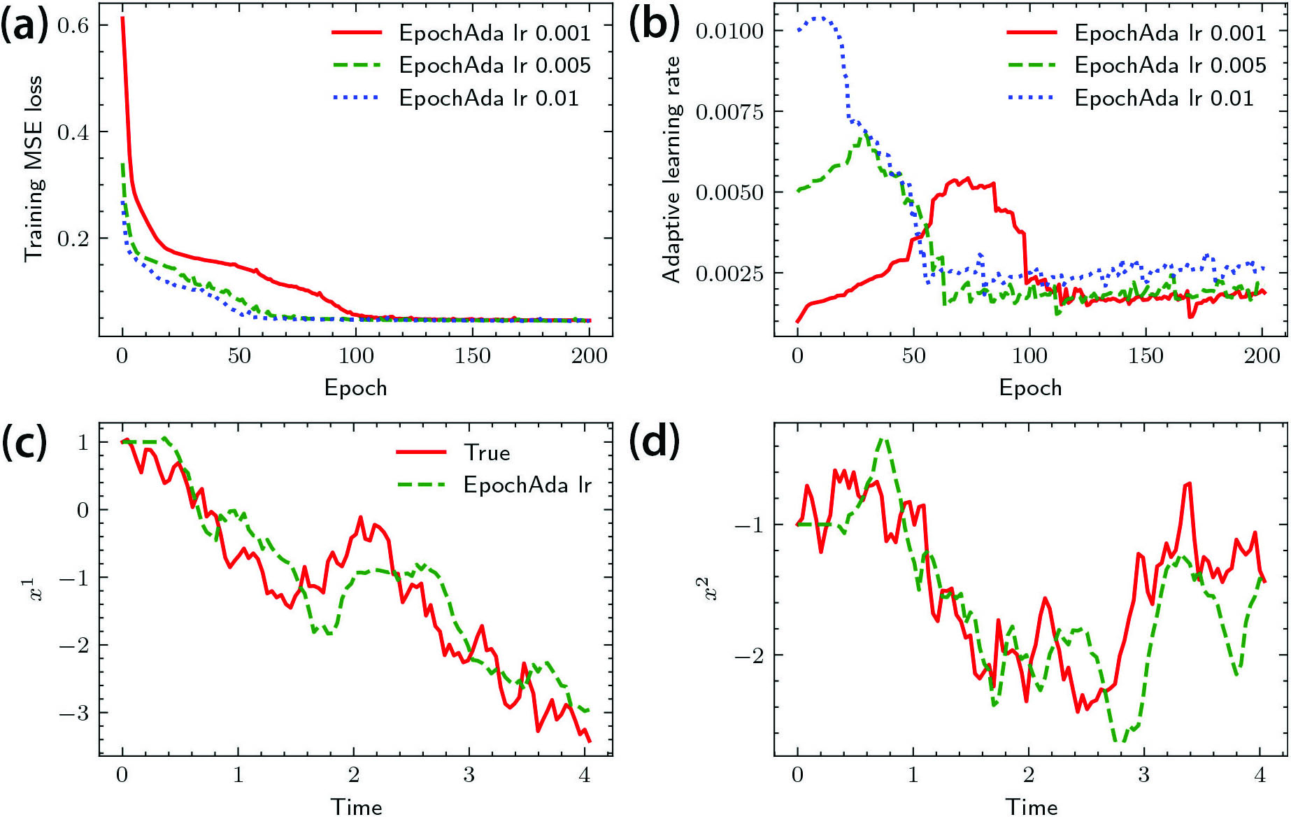
Example 1: Consider a two-dimensional (2D) nonlinear system with sinusoidal nonlinearity and a Markov switching process; the state and observation variables \(x\) and \(y\) are both 2D. According to the computational results in Figure 2, the performance in terms of relative errors is robust with respect to the initial learning rates.

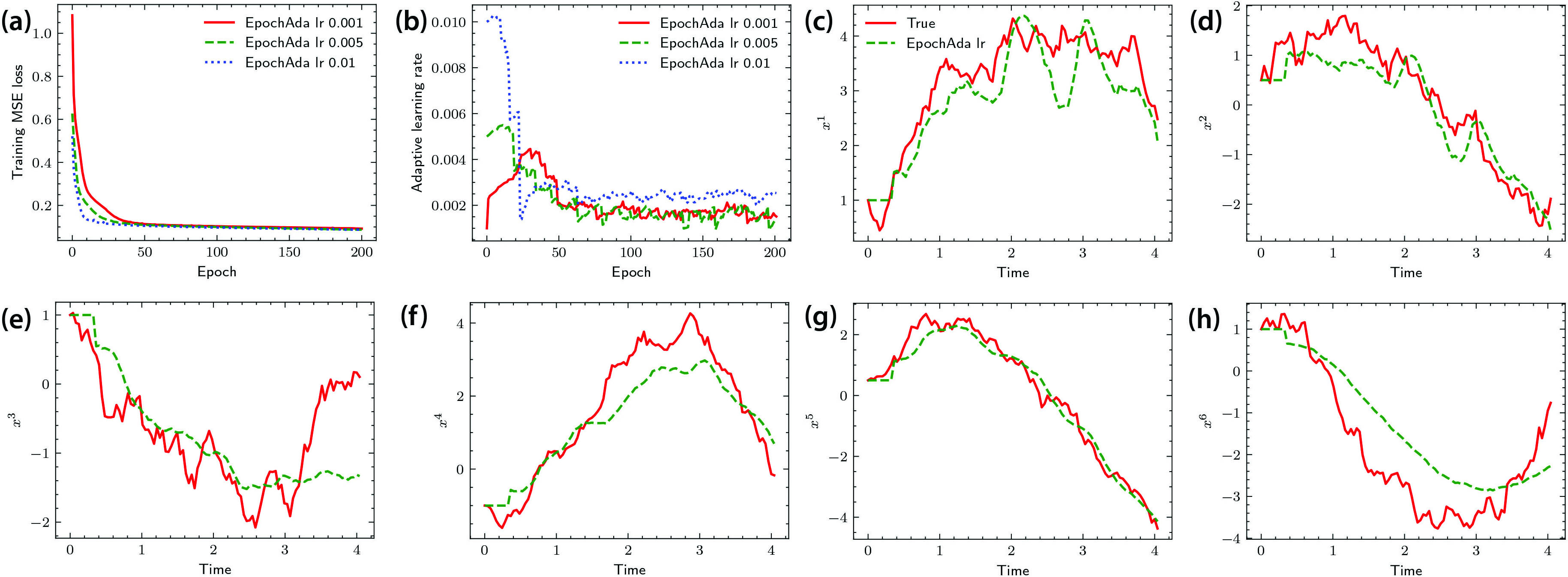
Example 2: Motivated by a target tracking problem, consider a six-dimensional dynamical system of a 2D moving particle. In the observation equation for this scenario, the first two components respectively represent the distance and angle. Figure 3 displays the numerical results.

Conclusions

We have presented a new computational method to solve challenging nonlinear filtering problems. Now we conclude with a few observations:

(i) Filtering that involves random switching is difficult. There is no easy way out or ready-made method from the computational toolbox. Our deep filtering algorithm serves as an effective procedure.

(ii) Although the algorithm targets nonlinear filtering, it is applicable to linear systems as well. We have conducted numerical experiments for linear systems and compared them with optimal Kalman filters, noting that the Kalman filters heavily depend on the type of nominal models in question. Such dependence is less pronounced with deep filtering.

(iii) Nonlinear filtering computations often break down when treating functions that involve sinusoidal signals. Deep filters can handle these signals with no substantial difficulty. 

(iv) Sparsity in the model may render undesirable outputs. In such a case, one can utilize a deep filter together with several regularization procedures. 

(v) In switching diffusions, the use of a deep filter can help devise a computational procedure if the Markov chain is also part of the state to be restored. Though it is currently possible to carry out the computation, the accuracy needs further improvement.

Our computational filtering method, which is based on deep learning techniques, unlocks new avenues for the solution of numerous problems that require the computation and estimation of unknown system signals. This article reports on a straightforward implementation, and we welcome suggestions to improve the overall performance or modify and enhance the basic algorithms.

References

[1] Duncan, T.E. (1967). Probability densities for diffusion processes with applications to nonlinear filtering theory and detection theory [Ph.D. dissertation, Department of Electrical Engineering, Stanford University]. Stanford University ProQuest Dissertations Publishing.
[2] Kloeden, P.E., & Platen, E. (1992). Numerical solution of stochastic differential equations. Berlin, Germany: Springer-Verlag.
[3] Kushner, H.J. (1964). On the differential equations satisfied by conditional probability densities of Markov processes, with applications. J. SIAM Ser. A Control, 2(1), 106-119.
[4] Kushner, H.J., & Yin, G. (2003). Stochastic approximation and recursive algorithms and applications (2nd ed.). New York, NY: Springer.
[5] Lototsky, S., Mikulevicius, R., & Rozovskii, B.L. (1997). Nonlinear filtering revisited: A spectral approach. SIAM J. Control Optim., 35(2), 435-461.
[6] Mortensen, R.E. (1968). Maximum-likelihood recursive nonlinear filtering. J. Optim. Theory Appl., 2, 386-394.
[7] Qian, H., Yin, G., & Zhang, Q. (2023). Deep filtering with adaptive learning rates. IEEE Trans. Automat. Control, 68(6), to appear.
[8] Shiryaev, A.N. (1966). On stochastic equations in the theory of conditional Markov processes. Theory Probab. Appl., 11, 179-184.
[9] Stratonovich, R.L. (1960). Conditional Markov processes. Theory Probab. Appl., 5(2), 156-178.
[10] Zakai, M. (1969). On the optimal filtering of diffusion processes. Z. Wahrsch. Verw. Gebiete., 11, 230-243.