Characterizations of Double Descent

Double descent is a machine learning (ML) phenomenon that pertains to an unexpected decline in test set errors during the creation of a sequence of increasingly overparameterized models. This behavior is vital to the success of modern generative models for image, video, and text because it allows them to generalize beyond their training data to seemingly new samples. Theorists are especially interested in double descent, as it seems to contradict conventional wisdom in applied mathematics and statistical learning. While the ML community often credits implicit regularization as the mechanism that enables overparameterized models, double descent can appear beyond this overparameterization in several ways.

Because researchers can suppress or manipulate double descent in numerical studies, the technique continues to inspire mathematical analysis. The Third Joint SIAM/CAIMS Annual Meetings (AN25), which took place this summer in Montréal, Québec, Canada, featured a two-part minisymposium titled “Double Descent and Related Phenomena in Modern Statistical Learning.” The session addressed theoretical frameworks and experiments with both synthetic and real problems, as well as broader perspectives on this theme.

A Minimal Working Example

The simplest demonstration of double descent relates to a common topic in numerical analysis. Let us describe an existing numerical experiment [3] with an associated minimal working example in MATLAB (see Figure 1b). Specifically, we seek a polynomial to fit a set of \(n\) points \((x_i, y_i) \in \mathbb{R}^2\) in the sense of ordinary least squares; an optimal polynomial minimizes \(\sum_{i=1}^n (p_k(x_i) - y_i)^2,\) where \(p_k(x)\) is a polynomial of degree \(k\). The problem reduces to a linear system \(A \theta = y\), and the “backslash” operator in MATLAB stably implements the solution \(\theta^* = A^\dagger y\) for any compatible matrix \(A\). What degree \(k\) should we choose? A polynomial of degree \(n-1\) is sufficient in exact arithmetic, but it is sensitive to data perturbations like floating-point roundoff or measurement error. Even if the “law” that underlies the data is a low-degree polynomial, this sensitivity yields fitted polynomials with wild oscillations in the interior of the domain. Such an outcome explains the conventional wisdom to prescribe a polynomial degree \(k \ll n\) rather than \(k=n-1,\) and certainly not \(k>n.\) Larger degree polynomials do not behave well with extrapolation—or even with interpolation on unseen data—when oscillations begin to appear.

Ignoring this conventional wisdom reveals double descent, where increasing \(k\) well past the underparameterized regime \((k<n)\) results in a model that generalizes by regressing unseen data — as evidenced when the test set error returns to values that are comparable to those in the underparameterized regime. In Figure 1a, the training set error approaches \(\varepsilon_\textrm{mach}\) at a predictable pace; at the same time, the test set error first increases, then—for sufficiently large \(k>n\)—is comparable to when \(k \ll n.\) The overparameterized polynomial provides some insight about the activity within this regime (see Figure 1a).

How does this phenomenon occur? Can we control or suppress it? The presentations in the AN25 minisymposium offered a variety of perspectives through which we can understand and control the appearance of such peaks in the loss of a model, and describe and connect related phenomena.

Tunable Double Descent in Large-data, Large-parameter Limits

Rishi Sonthalia of Boston College considered the question of double descent from a probabilistic perspective. He analyzed a similar linear regression task for learning \(\theta\) in the relationship \(y = \theta^T x + \xi,\) where \(x \in \mathbb{R}^d\) is sampled \(N(0,I)\) and \(\xi\) represents independent, normally distributed noise. While linear regression is a far cry from neural networks, Sonthalia’s framework utilizes tools from random matrix theory to analyze the data matrix \(X\) and fitted parameters \(\hat{\theta}\) as a function of \(d\) and the number of data samples \(n.\) Curiously, the generalization risk \(\mathcal{R} = E[ ((\theta^* - \hat{\theta})^T x)^2]\) in the joint large-data, large-parameter limit \(c=d/n\) is actually a piecewise function of \(c\) with a simple pole at \(c=1.\) This is a model of the phenomenon, but it cannot explain the variety of real-world behavior.

To add an element of control to the situation, Sonthalia proposed two approaches to regulate the peak in empirical risk relative to \(c\) [2]. The first approach involves data that was sampled from a mixture of two Gaussian distributions: (i) an isotropic Gaussian, sampled with probability \(\pi,\) and (ii) a one-dimensional Gaussian, sampled from rank-one subspace \(\textrm{span}(z)\) with probability \(1-\pi.\) By following this design, Sonthalia finds a generalization risk 

\[\mathcal{R} = \left\{ \begin{array}{ll} 
\frac{\pi c}{\pi - c}, & c<\pi, \\
\pi \left( \frac{\pi}{c-\pi}+ C(d,z) \left( 1- \frac{\pi}{c}  \right) \right), & c > \pi.
\end{array} \right.\]

The risk asymptotes at value \(c=\pi \leq 1,\) which means that it will contradict the classical interpolation threshold of \(c=1.\) As such, it can be made to appear arbitrarily early in the underparameterized regime.

Sonthalia’s second approach implements a more practically relevant regularized least squares method with regularization parameter \(\mu\) and a sophisticated design for data distribution, with multiple additional parameters to \(n,\) \(d,\) and \(c=d/n.\) While the full risk expression is quite complicated, \(\mathcal{R}\) peaks at \(c=1/(1+\mu^2)\) in a simple setting. Risk peaks at the interpolation threshold \(c=1\) when \(\mu=0;\) when \(\mu>0,\) however, Sonthalia can push this peak towards \(c=0\) (the underparameterized regime).

Ultimately, Sonthalia’s analysis reveals that double descent can occur even in the underparameterized regime—and with regularization in the loss—and is disconnected from other plausible explanations, such as the operator norm of the estimator for \(\theta.\)

Double Descent in Training and Scale-time Equivalence

During his presentation, Akhilan Boopathy of Kuai identified specific scenarios wherein a “double descent in time” transpires during training and can be explained based on the concept of scale-time equivalence. A key observation pertains to the ability to observe and control double descent throughout the training process. Consider a binary classifier: a function \(f: \mathbb{R}^n \to \{0,1\}.\) For most binary classification tasks with “big” and “small” data, minor perturbations to the data do not significantly affect the resulting decision boundary — a concept that is key to the formulation of support vector machines.

However, Boopathy argues that the interpolation regime is sensitive to small perturbations with respect to directions of low variance in the data. Using this perspective, he broadens the sense of an interpolation threshold to include the moment when a model that is being trained first “discovers” all directions of variance in the data. This incidence may arise at the classical threshold \(n=d,\) but it can also occur elsewhere depending on the nature of the data and model.

Boopathy and his collaborator, Ila Fiete of the Massachusetts Institute of Technology, harness projectors to bridge the gaps between model size, trainable space, and directly controllable parameters [1]. They implement these ingredients in a toy model that is based on random subspaces. First, they train a model with \(n\) parameters whose outputs depend on subspace dimension \(r;\) here, \(p\) of the model parameters are controllable, with \(r<p<n.\) A linear projector \(K\) sends the original parameters \(\beta \in \mathbb{R}^n\) to parameters \(\alpha \in \mathbb{R}^r,\) and the model is fit to discover \(\beta\) by trainable parameters \(\theta \in \mathbb{R}^p.\)

Boothpathy and Fiete demonstrated the formation of the following projected gradient flow problem for a smooth loss function \(L\) on \(\alpha\):

\[\begin{eqnarray}\frac{d A_t}{dt} &=& - \eta K K^T \nabla L(A_t), \\ A_0 &=& K \beta_0. \end{eqnarray}\]

Here, the norm \(|| \alpha_t – A_{pt}||\)—which depends on the joint quantity \(pt,\) among other terms—can be bounded. Researchers can thus relate the practically trainable \(\alpha_T\) with \(r\) parameters to models \(A_{T}\) with \(r\) parameters, but also to \(A_{2T}\) with \(r/2\) parameters or \(A_{T/2}\) with \(2r\) parameters.

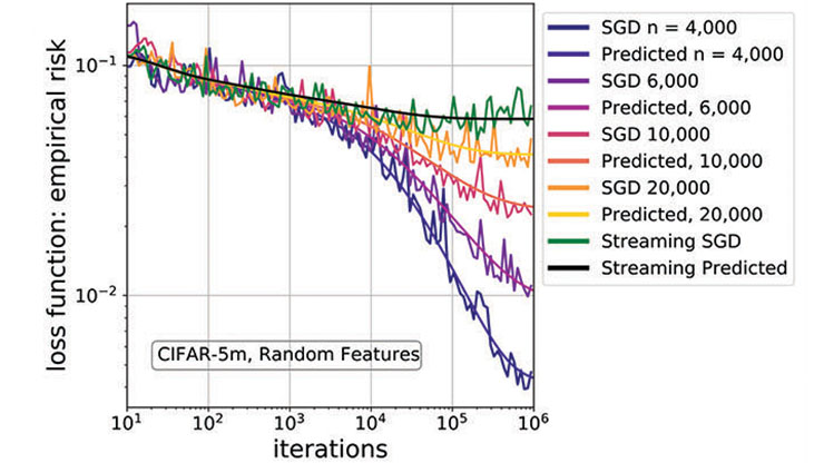
Moving beyond nested linear-affine models, Boopathy and Fiete also used a family of convolutional neural networks to test scale-time equivalence on an image classification task and found an empirical scaling law that showed good agreement with their hypothesis (see Figure 2). The implications of scale-time equivalence are striking, suggesting that larger models require fewer epochs to generalize than smaller models. This equivalence also cleanly connects parameter-wise and epoch-wise double descent theory.

Double Descent as a Manifestation of the Generalized Aliasing Decomposition

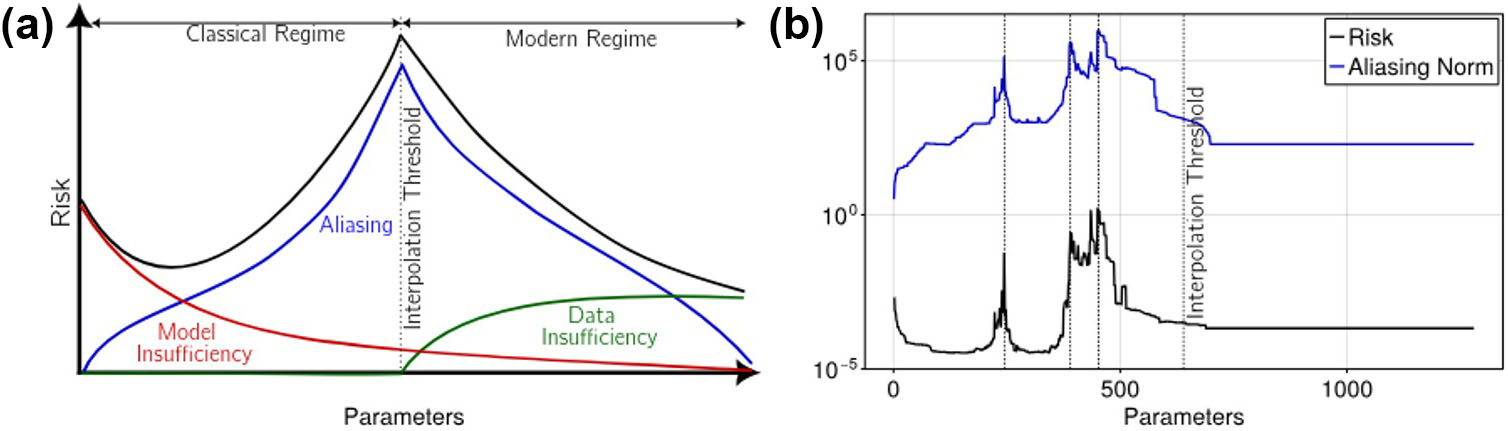
Tyler Jarvis—in collaboration with Mark Transtrum, Gus Hart, and Jared Whitehead, all of Brigham Young University—presented a third view of double descent and took a functional-theoretic approach with their generalized aliasing decomposition [5]. This technique is inspired by the classical signal processing phenomenon of mistaking an undersampled, high-frequency sinusoid for one with a lower frequency. The team motivated their work with an application in materials science that exhibits multiple peaks prior to the classical interpolation threshold (see Figure 3b).

From the lens of function approximation, Jarvis and his colleagues assumed a complete set of model functions \(\Phi_j : \Omega \to \mathbb{R}\) so that convergent series \(y(t) = \sum_{j} \Phi_j(t) \theta_j\) describes the true function \(y(t)\) for approximation. Then, \(\mathbf{y} = \mathbf{M}\theta\) for a bounded linear operator \(\mathbf{M},\) which maps parameter space \(\Theta\) to data space \(\mathcal{D}.\) In this setting, the researchers decomposed model space \(\Theta\) into modeled and unmodeled components \(\mathcal{M} \oplus \mathcal{U},\) and data space \(\mathcal{D}\) into training and prediction \(\mathcal{T} \oplus \mathcal{P}.\) They analyzed this block operator and identified three contributions to model risk: model insufficiency, data insufficiency, and aliasing.

This aliasing—which is expressible as \(A = \mathbf{M}_{\mathcal{TM}}^{+} \mathbf{M}_{\mathcal{TU}}\) and related to a block decomposition with modeled and unmodeled components of the operator \(\mathbf{M}\)—has operator norm \(||A||,\) whose value explains the classical interpolation threshold peak in synthetic experiments (similar to Figure 3a), the multiple peaks in their original application (see Figure 3b), and other standard nonlinear ML problems.

Reflections

Ultimately, the AN25 minisymposium captured myriad ways to describe, analyze, and control the unique phenomenon of double descent. Several other viewpoints—including the information-theoretic perspective of Vapnik-Chervonenkis theory, the use of sharpness-aware minimization to improve generalizability, and a philosophical and scientific take on double descent—offered important critiques and comments on the ML community and scientific process at large. Given the many subtleties and bridges between theory and application, it is naive to think of double descent as a phenomenon in which a single framework dominates. Rather, we should view it as distinct perspectives that provide guidance under different settings. I look forward to the field’s continued evolution and the ultimate transformation of theory into action.

References 
[1] Boopathy, A., & Fiete, I. (2024). Unified neural network scaling laws and scale-time equivalence. Preprint, arXiv:2409.05782.
[2] Li, X., & Sonthalia, R. (2024). Least squares regression can exhibit under-parameterized double descent. In NIPS ‘24: Proceedings of the 38th international conference on neural information processing systems (pp. 25510-25560). Vancouver, Canada: Curran Associates Inc.
[3] Schaeffer, R., Khona, M., Robertson, Z., Boopathy, A., Pistunova, K., Rocks, J.W., … Koyejo, O. (2023). Double descent demystified: Identifying, interpreting and ablating the sources of a deep learning puzzle. Preprint, arXiv:2303.14151.
[4] Schaeffer, R., Robertson, Z., Boopathy, A., Khona, M., Pistunova, K., Rocks, J.W., … Koyejo, S. (2023). Double descent demystified: Identifying, interpreting and ablating the sources of a deep learning puzzle. Retrieved from https://github.com/RylanSchaeffer/Stanford-AI-Alignment-Double-Descent-Tutorial.
[5] Transtrum, M.K., Hart, G.L.W., Jarvis, T.J., & Whitehead, J.P. (2025). Generalized aliasing explains double descent and informs model design. Phys. Rev. Res., to be published.