Control and Machine Learning

Two recurring questions pertain to the origin, history, and present state of mathematics. The first relates to math’s incredible ability to describe natural, industrial, and technological processes, while the second concerns the unity and interconnectedness of all mathematical disciplines. Here I describe some of the gateways that link two particular mathematical branches: control theory and machine learning (ML). These areas, both of which have very high technological impacts, comprise neighboring valleys in the complex landscape of the mathematics universe.

Control theory certainly lies at the pedestal of ML. Aristotle anticipated control theory when he described the need for automated processes to free human beings from their heaviest tasks [3]. In the 1940s, mathematician and philosopher Norbert Wiener redefined the term “cybernetics”—which was previously coined by André-Marie Ampère—as “the science of communication and control in animals and machines,” which reflected the discipline’s definitive contribution to the industrial revolution.

Wiener’s definition involves two essential conceptual binomials. The first is control-communication: the need for sufficient and quality information about a system’s state to make the right decisions, reach a given objective, or avoid risky regimes. The second binomial is animal-machine. As Aristotle predicted, human beings rationally aim to build machines that perform tasks that would otherwise prevent them from dedicating time and energy to more significant activities. The close link between control and/or cybernetics and ML is thus built into Wiener’s own definition.

The interconnections between different mathematical disciplines are split by conceptual and technical mountain ranges and have often evolved in different communities. As such, they are frequently hard to observe. Building the connecting paths and identifying the hypothetical mountain passes requires an important level of abstraction. Let us take a step back and consider a wider perspective.

The notion of controllability helps us disclose one of the gateways between disciplines. Controllability involves driving a dynamical system from an initial configuration to a final one within a given time horizon via skillfully designed and viable controls. In the framework of linear finite \(N\)-dimensional systems

\[x'+Ax=Bu,\]

the answer is elementary and classical (it dates back to Rudolf Kalman’s work in the 1950s, at least) [6]. The system is controllable if and only if the matrix \(A\) that governs the system’s dynamics and the matrix \(B\) that describes the controls’ effects on the state’s different components verify the celebrated rank condition

\[\textrm{rank}[B,AB,...A^{N-1}B]=N.\]

The control’s size naturally depends on the length of the time horizon; it must be enormous for very short time horizons and can have a smaller amplitude for longer ones.

In fact, as John von Neumann anticipated and Nobel Prize-winning economist Paul Samuelson further analyzed, the “turnpike” property manifests itself over long time horizons; controls tend to spend most of their time in the optimal steady-state configuration [5]. We apply this lesser-known principle systematically (and often unconsciously) in our daily lives. When travelling to work, for instance, we may rush to the station to take the train—our turnpike in this ride—on which we then wait to reach our final destination. Medical therapies for chronic diseases also utilize this principle; physicians may instruct patients to take one pill a day after breakfast, rather than follow a sharper but much more complicated dosage. This property even arises in the field of economics when national banks set interest rates in six-month horizons and only revisit the policies to adjust for newly emerging macroeconomic scenarios.

Are these ideas and methods at all relevant to ML? Let us start with George Cybenko’s seminal result: the so-called universal approximation theorem (UAT). The UAT states that a finite combination of rescaled and shifted activation functions (i.e., neural networks) are dense in a variety of functional classes [1]. This functional analysis result complements other fundamental outcomes in analysis, including the density of polynomials, Fourier series, and compactly supported smooth functions.

The UAT serves regression and classification purposes in the context of supervised learning (SL). Roughly, we can classify any data set by simply approximating the characteristic function—taking value \(1\) in one set of items and \(0\) in the complementary one—to ultimately allocate the correct label to each item.

Cybenko’s beautiful result, which was proven as a corollary of the Hahn-Banach theorem, opened the door for a variety of methods that now play an essential role in ML. Because the UAT guarantees the achievement of all goals by simply identifying the right parameters in Cybenko’s ansatz

\[f(x)=\sum^n_{k=1}W_k\sigma(A_k \cdot x+ b_k),\]

we may adopt the least squares point of view and search for parameter values that minimize the distance to the needed function during the so-called training phase. Of course, such a naive and natural approach leads to great challenges — we must simultaneously face the devil of the lack of convexity and the curse of dimensionality!

Eduardo Sontag and Hector Sussmann explored the control consequences of dynamical systems properties of the form

\[\dot{x}(t)=W(t)\sigma(A(t) \cdot x(t)+b(t)), \quad t \ge 0,\]

a concept that Weinan E later revisited [2, 9]. This form is a neural ordinary differential equation (NODE) that is driven by activation functions \(\sigma\), like the sigmoid functions (monotonic continuous functions that take value \(0\) at \(-\infty\) and \(1\) at \(+\infty\)). Cybenko introduced these functions—which are rather atypical in mechanics—for approximation purposes.

It took the mathematical control community many years to understand how to apply control methods to the real challenges of SL. Recent works have finally proved that deep residual neural networks (ResNets)—time discretizations of NODEs—enjoy the amazing and unexpected property of simultaneous or ensemble control [8]. We can build controls (i.e., train parameters) in such a way that an arbitrarily large number of trajectories simultaneously arrive almost exactly at their targets: the labels that correspond to the items of the data set to be classified (see Figure 1).

This dynamical systems perspective presents some interesting advantages by offering better dependence of available data and the opportunity to tune classification methods for improved stability properties. It can also exploit plenty of the existing knowledge in more mature areas of applied mathematics. In fact, the activation function \(\sigma\)’s very nature is responsible for the exceptionally powerful property of simultaneous control that ensures the requirements of SL. The most paradigmatic example is the Rectified Linear Unit (ReLU) activation function, which simply takes the value \(0\) when \(x<0\) and \(1\) when \(x>0\). When driven by the ReLU, a NODE behaves like a Rubik’s Cube — it is solvable via a finite number of smart operations for which part of the cube is frozen while the other part rotates in the appropriate direction and sense. The goal of a Rubik’s Cube is to ensure that all faces are homogeneous in color. This objective is similar to the task of a NODE, which drives each initial item to a given distinguished reservoir according to its label.

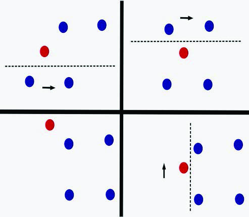
The proofs in previous studies are inductive, and researchers build the controls (or parameters) to be piecewise constant in order to exploit the ReLU’s essence [8]. At each time instant, the ReLU splits the Euclidean space into two half-spaces: (i) one that is frozen along the dynamics because the nonlinearity vanishes and (ii) one that evolves exponentially where the ReLU is active. A strategic, inductive choice of the different hyperplanes/equators (via selection of the values of the controls/parameters \(A\) and \(b\)) and the direction of the dynamics/wind (via the control \(W\)) guarantees classification in a finite number of steps (see Figure 2).

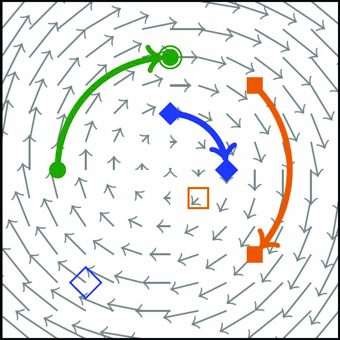
These results provide the backbone theory to ensure that NODEs fulfill the ensemble controllability properties that are necessary for classification. Of course, the controls that we observe in numerical simulations are often less complex, since they are computed as minimizers of a suitably penalized loss functional. Such findings rely fundamentally on the nonlinearity of the activation functions \(\sigma\). Indeed, the ensemble controllability property is impossible for a linear system that would rather behave like the system in Figure 3, unable to classify items according to labels.

We can transfer this control result for ResNets and NODEs to the framework of transport equations (advection, convection, and so forth) via the classical principle that the trajectories of the first equations constitute the characteristics of the latter:

\[x'(t)=\sigma(x(t),t) \rightarrow \partial_t v + \textrm{div}_x(\sigma(x,t)v)=0.\]

Approximating the distributions of masses to be transported with atomic measures—whose supports play the role of items in classification—accomplishes this transfer. Control and ML also come together in the traditional problem of mass transport, though not exactly in the same way as in optimal transport or the Monge-Kantorovich problem. Rather, these disciplines align by means of time-dependent vector fields with the oversimplified geometry of the activation function.

My colleagues and I are not the first researchers to claim the tight connections between control and ML [4, 7]. But now that we have been working on this topic for several years, we realize that there is still much to discover in the vast forest that connects these two areas. Although finding the paths through the dense grove will be intellectually challenging, doing so may add additional detail to the fascinating global map of the mathematical sciences. These paths will likely take a zigzagged course that resembles the strategies for solving a Rubik’s Cube or the trajectories that assure the needs of learning through ResNet control.

Many other unexplored realms merit the attention of the applied mathematics community as well. One such topic is federated learning — a subject that is closely related to the classical splitting and domain decomposition methods in numerical analysis. We are currently investigating federated learning in cooperation with the artificial intelligence company Sherpa.ai, but we leave this topic for another occasion.

This article is based on Enrique Zuazua’s W.T. and Idalia Reid Prize Lecture at the 2022 SIAM Annual Meeting, which took place this July in Pittsburgh, Pa. 

References

[1] Cybenko, G. (1989). Approximation by superpositions of a single function. Math. Control Signals Syst., 2, 303-314.
[2] E, W. (2017). A proposal on machine learning via dynamical systems. Commun. Math. Stat., 5, 1-11.
[3] Fernández-Cara, E., & Zuazua, E. (2003). Control theory: History, mathematical achievements and perspectives. Bol. Soc. Esp. Mat. Apl., 26, 79-140.
[4] Fradkov, A.L. (2020). Early history of machine learning. IFAC-PapersOnLine, 53(2), 1385-1390.
[5] Geshkovski, B., & Zuazua, E. (2022). Turnpike in optimal control of PDEs, ResNets, and beyond. Acta Numer., 31, 135-263.
[6] Kalman, R.E. (1960). On the general theory of control systems. IFAC Proc. Vol., 1(1), 491-502.
[7] LeCun, Y. (1988). A theoretical framework for back-propagation. In D. Touretzky, G.E. Hinton, & T. Sejnowski (Eds.), Proceedings of the 1988 connectionist models summer school (pp. 21-28). Pittsburgh, PA: Carnegie Mellon University.
[8] Ruiz-Balet, D., & Zuazua, E. (2021). Neural ODE control for classification, approximation and transport. Preprint, arXiv:2104.05278. 
[9] Sontag, E., & Sussmann, H. (1997). Complete controllability of continuous-time recurrent neural networks. Syst. Control Lett., 30(4), 177-183.