Factorizations for Data Analysis

Factorization breaks an object into building blocks that we can understand and interpret: e.g., a number into primes, a variety into irreducible components, or a matrix into rank-one summands. This process underpins classical paradigms for data analysis, including principal component analysis (PCA) via the eigendecomposition. But because modern datasets record information from various contexts and modalities, classical factorizations can no longer sufficiently analyze them. Can new factorizations hold the key to human-interpretable understanding of today’s complex systems?

Mathematically, the challenge involves the factorization of an interconnected collection of matrices or tensors, which is achievable through algebraic insights. Here, I will overview three classical factorizations in traditional data analysis tools and then present two new factorizations for the analysis of multi-context data.

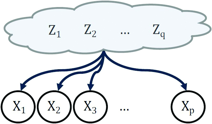
The following is a general framework for data analysis. We model observed random variables \(X\) as an unknown mixture of unknown latent (unobserved) random variables \(Z\) (see Figure 1). When the mixture occurs via a linear map \(A\), then \(X=AZ\). The factors \(A\) and \(Z\) are both unknown.

Our goal is to recover the mixing matrix \(A\) and latent variables \(Z\) from samples of \(X\). The building blocks \(A\) and \(Z\) define components that explain structures in the data — for example, identifying gene modules in gene expression data, separating signal from artifacts (such as eye blinks) in electroencephalogram data, and providing axes for visualization in dimensionality reduction.

We recover the latent variables \(Z\) and mixing map \(A\) by turning the relationship \(X=AZ\) into a factorization problem. The first cumulant of \(X\) is its mean and the second is its covariance: the \(p \times p\) positive semidefinite matrix \(\Sigma_X\) that records at entry \((i,j)\) the way in which variables \(X_i\) and \(X_j\) vary together. The relationship \(X=AZ\) implies that the covariance matrices of \(X\) and \(Z\) relate via congruence action

\[\Sigma_X=A\Sigma_ZA^{ \top}.\]

When \(\Sigma_X\) is known and \(\Sigma_Z\) and \(A\) are unknown, this is a matrix factorization problem. In practice, we do not have access to the true \(\Sigma_X\) and instead work with the sample covariance matrix,¹ which is denoted by \(S\). Classical data analysis tools live in this factorization framework, as I will demonstrate next.

PCA Is the Eigendecomposition

In PCA, observed variables are an orthogonal transformation of uncorrelated latent variables (see Figure 2a). So 

\[S= V\,DV^{ \top},\]

where the columns of \(V\) are the principal components—which express each latent variable as a linear combination of observed variables—and \(D\) is a diagonal matrix that records the variance of the latent variables. The eigendecomposition proves that a real symmetric matrix has such a factorization (\(V\) is the matrix of eigenvectors and \(D\) is their eigenvalues), and that it is unique for general \(S\).

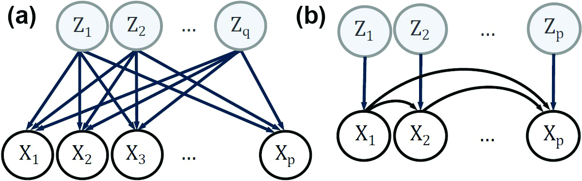
Linear Structural Equation Models Are the LDL Decomposition

We can model variables \(X\) to relate via noisy linear dependencies: \(X= B X+Z\) (see Figure 2b). In such a linear structural equation model (LSEM), \(b_{ij}\) is the effect of variable \(X_j\) on \(X_i\) and \(Z\) is a vector of exogenous noise variables (typically assumed to be independent) [10]. We usually further assume that the dependencies follow a directed acyclic graph, where \(b_{ij}=0\) unless \(j \rightarrow i\) is an edge in the graph. It is then possible to reorder the variables to make \(B\) strictly lower triangular. We obtain \(X=AZ\) for \(A=(I-B)^{-1}\) and hence

\[S=(I-B)^{-1}D(I-B)^{-\top},\]

where \(D\) records the variances of the latent variables. This is the LDL decomposition.

In both of the previous examples, the latent variables have diagonal covariance because they are uncorrelated. But the factorization \(ADA^{\top}\) would not be unique without an additional structure on \(A\), which is orthogonal in PCA and becomes lower triangular in the LSEM. This extra structure makes the factorization unique; the uniqueness of the eigenvectors \(\mathbf{v}\) or weights \(b_{ij}\) aids downstream analysis.

I have only focused on covariance thus far, but a distribution has a \(d\)th cumulant² \(\kappa_d(X)\) for any positive integer \(d\). If \(X=AZ\), then the cumulants relate via a higher-order congruence action 

\[\kappa_d(X)=A\bullet \kappa_d(Z),\]

which specializes to matrix congruence when \(d=2\). For the \(p \times p \times p \times p\) cumulant (i.e., kurtosis tensor), the \((i,j,k,l)\) entry of \(\kappa_4(X)\) is \(\sum^q_{i',j',k',l'=1} \, a_{ii'}a_{jj'}a_{kk'}a_{ll'}(\kappa_4(Z))_{i'j'k'l'}\). The tensor \(\kappa_d(X)\) is known (or estimated from data), while \(A\) and \(Z\) are unknown. This is now a tensor factorization.

Independent Component Analysis Is Symmetric Tensor Decomposition

Independent variables have diagonal cumulants. If \(X=AZ\) for independent variables \(Z_i\), then the congruence transformation yields

\[\kappa_d(X)=\sum^q_{i=1}\lambda_i \mathbf{a}_i^{\otimes d},\]

where \(\mathbf{a}_i\) is the \(i\)th column of \(A\) and \(\lambda_i\) is the \(d\)th cumulant of \(Z_i\). This is the usual symmetric tensor factorization. Under the correspondence between symmetric tensors and homogeneous polynomials, the factorization seeks to decompose a polynomial into a sum of powers of linear forms — a method that dates back to the 19th century [7]. We can impose additional structure on \(A\), such as orthogonality [11] or \(A=(I-\Lambda)^{-1}\) [5], but doing so is not required; the uniqueness of tensor factorization [1] makes independent component analysis (ICA) identifiable for general matrices \(A\), including in the “overcomplete” case when \(q>p\) [2, 3, 9].

We have now explored the factorizations behind three classical tools. In present-day experiments, we aim to understand systems by collecting data across a range of contexts. This process requires new factorizations, as evidenced by the following two examples.

Linear Causal Disentanglement Is the Partial Order QR Decomposition

The three preceding methods assume uncorrelated latent variables. In contrast, causal disentanglement is an area of machine learning that seeks latent variables with causal dependencies between them. In linear causal disentanglement (LCD), observed variables \(X\) are a linear transformation of latent variables \(Z\) that follow an LSEM (see Figure 3a) [6]. The covariance therefore has factorization

\[\Sigma_X=A(I-B)^{-1}D(I-B)^{-\top}A^{\top}.\]

Too many parameters exist for unique recovery from \(\Sigma_X\). Instead, LCD is appropriate for data that are observed under multiple contexts that are related via interventions on a latent variable. We characterize the number of required contexts for identifiability and provide an algorithm to recover the parameters. To do so, we define the partial order QR factorization: a version of the QR factorization³ for matrices whose columns observe a partial order rather than the usual total order.

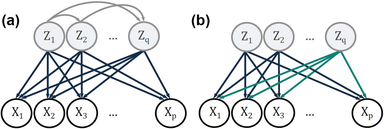
Contrastive ICA Is Coupled Tensor Decomposition

To describe a foreground dataset (i.e., an experimental group) relative to a background dataset (i.e., a control group), we attempt to jointly model variables across the two contexts. In contrastive ICA [8], we model the foreground and background as two related ICA models (see Figure 3b). The \(d\)th cumulants of the foreground and background are respectively

\[\sum^q_{i=1}\lambda'_i \mathbf{a}_i^{\otimes d} + \sum^r_{i=1} \mu_i \mathbf{b}_i^{\otimes d} \qquad \textrm{and} \qquad \sum^q_{i=1}\lambda_i \mathbf{a}_i^{\otimes d}.\]

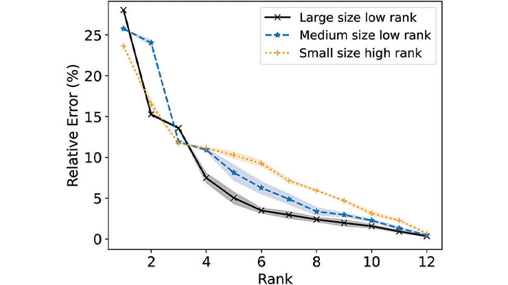
We jointly factorize the two cumulant tensors. For matrices, we can always take a best low-rank approximation as a sum of orthogonal terms. However, this is no longer true for tensors; we must find a tradeoff between accuracy and orthogonality. We first use the subspace power method [4] for accuracy, then incorporate a new hierarchical tensor decomposition for orthogonality.

As datasets continue to increase in richness, their complexity presents an opportunity for mathematicians to reveal the structure in modern data by advancing and applying the mathematics of factorizations. There are many open directions, including the development of linear and multilinear algebra ideas to establish the existence and uniqueness of new factorizations, sample complexity investigations, numerical algorithms, and extensions to nonlinear transformations.

¹ For mean-centered data \(\mathbf{x}^{(1)},...,\mathbf{x}^{(n)} \in \mathbb{R}^p\), the sample covariance is the average of the outer products of the data points: \(S=\tfrac{1}{n}\sum_i \mathbf{x}^{(i)} \mathbf{x}^{(i)^\top}\).

² The \(d\)th order cumulant is the tensor of order \(d\) terms in \(\mathbf{t}=(t_1, …, t_p)\) in the cumulant-generating function \(\log\mathbb{E}(\exp(\mathbf{t}^{\top}X))\).

³ The QR factorization writes a matrix as the product of an orthogonal multiplied by an upper triangular matrix.

References
[1] Alexander, J., & Hirschowitz, A. (1995). Polynomial interpolation in several variables. J. Algebr. Geom., 4, 201-222.
[2] Comon, P. (1994). Independent component analysis, a new concept? Signal Process., 36(3), 287-314.
[3] Eriksson, J., & Koivunen, V. (2004). Identifiability, separability, and uniqueness of linear ICA models. IEEE Signal Process. Lett., 11(7), 601-604.
[4] Kileel, J., & Pereira, J.M. (2019). Subspace power method for symmetric tensor decomposition. Preprint, arXiv:1912.04007.
[5] Shimizu, S., Hoyer, P.O., Hyvärinen, A., & Kerminen, A. (2006). A linear non-Gaussian acyclic model for causal discovery. J. Mach. Learn. Res., 7(72), 2003-2030.
[6] Squires, C., Seigal, A., Bhate, S., & Uhler, C. (2023). Linear causal disentanglement via interventions. In ICML’23: Proceedings of the 40th international conference on machine learning (pp. 32540-32560). Honolulu, HI: Journal of Machine Learning Research.
[7] Sylvester, J.J. (1851). On a remarkable discovery in the theory of canonical forms and of hyperdeterminants. London Edinburgh Dublin Philos. Mag. J. Sci., 2(12), 391-410.
[8] Wang, K., Maraj, A., & Seigal, A. (2024). Contrastive independent component analysis. Preprint, arXiv:2407.02357.
[9] Wang, K., & Seigal, A. (2024). Identifiability of overcomplete independent component analysis. Preprint, arXiv:2401.14709.
[10] Wright, S. (1934). The method of path coefficients. Ann. Math. Stat., 5(3), 161-215.
[11] Zhang, T., & Golub, G.H. (2001). Rank-one approximation to high order tensors. SIAM J. Matrix Anal. Appl., 23(2), 534-550.