From Archimedes and Euclid to Hamilton and Poincaré

Symplectic maps of \({\mathbb R}  ^{2n}\) are basic objects of Hamiltonian mechanics, and the time \(t\) map of a Hamiltonian system’s position-momentum pair is symplectic. Symplectic maps of \({\mathbb R}  ^2\) are the area-preserving ones.

I recently realized that the Archimedian law of the lever amounts to an area-preservation property of a simple map of \({\mathbb R}  ^2\), as described next. Afterwards, I will reference an analogy between the Archimedian lever on the one hand and Hamiltonian mechanics on the other.

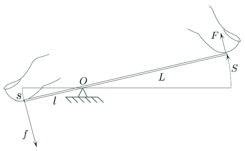
Figure 1 shows a seesaw in equilibrium, pressed at both ends. Archimedes’ law of the lever gives the condition for the equilibrium, \(fl=FL,\) i.e. 

\[F= \frac{l}{L} f.\]

Furthermore, \(S =  \frac{L}{l} s,\) according to Euclid. To summarize, we have the “Euclid-Archimedes map,” \((s,f)\mapsto (S,F)\), given by 

\[\begin{equation}  
   \left\{ \begin{array}{l} 
    S=   \lambda  s  \\ 
    F = \frac{1}{\lambda}  f,  \end{array} \right.    
\end{equation}  \tag1 \]

where \(\lambda = L/l\). This map is clearly area-preserving, but for a reason deeper than the explicit form \((1)\). Indeed, let us cyclically move the two fingers in Figure 1 so that the positions and the forces return to their original values. We end up doing zero work:

\[\oint f\,ds+ \oint (-F)\,dS=0, \tag2 \]

The minus sign is due to the fact that the right finger presses with force \(-F\). During the cyclic motion, the point \((s,f)\) describes a closed curve \(\gamma\) in the plane, while the point \((S,F)= \varphi (s,f)\) describes the image curve \(\varphi (\gamma )\). Therefore, the zero-work condition \((2)\) amounts to the equality of areas inside \(\gamma\) and \(\varphi (\gamma )\). Incidentally, \((2)\) is a compact way of saying that the lever is not a perpetual motion machine.

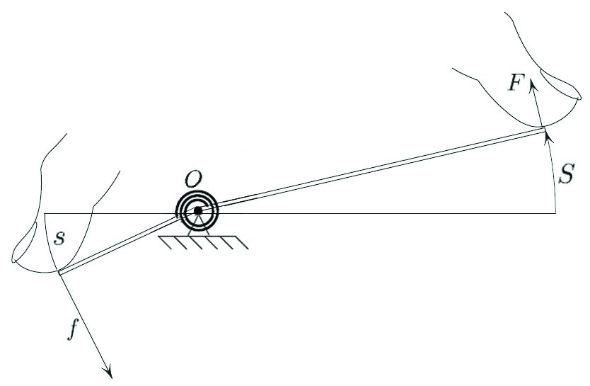
If the board can flex, as in Figure 2, then the map \((s,f)\mapsto (S,F)\) is no longer given by \((1)\), but is still area-preserving; the above proof applies without change. 

Seesaw and Hamiltonian Dynamics

Remarkably, the Hamiltonian flow is symplectic for the same reason that the “seesaw map” \(\varphi\) is area-preserving.¹ To make sense of the last sentence, I must specify the analogy between the seesaw in Figure 2 on the one hand and a Hamiltonian system on the other. The following explanation outlines this analogy (a full discussion can be found in [1]). Consider a mechanical system with the Lagrangian \(L,\) depending on generalized position and velocity. Let us fix two points \((0,q)\) and \((T,Q)\) in time-space and define the action \(A(q, Q) = \int_{0}^{T} L(r(t),\dot r(t)) \,dt \), with the integration occurring over the minimizer \(r(t)\) of the integral subject to \(r(0)=q\),  \(r(T)=Q\) (we assume this minimized is unique and depends smoothly on \(q,Q\)). For any (admissible) \(T\), the momenta \(p,P\) at times \(t=0\) and \(t=T\) are given by

\[ P = A_Q(q,Q), \  \  p =- A_q(q, Q). \tag3 \]

This can be taken as the definition of the momentum, or related (in a one-line calculation) to the more standard definition, as explained on page 261 of [1].

Returning now to the seesaw of Figure 2, let \(U(s,S)\) be the potential energy; then

\[F= U_S(s,S), \  \  f=- U_s(s,S). \tag4 \]

A comparison between \((3)\) and \((4)\) shows that the action and the momenta \((A, \  p, \  P)\) are close analogs of the potential energy and the forces \((U, \  f, \  F)\). The proof of the symplectic character of the time \(T\) map \((q,p) \mapsto (Q, P)\) for arbitrary \(T\) becomes a verbatim copy of the area preservation’s proof of the “seesaw map” \((s,f)\mapsto (S, F)\).

A Paradox

If the spring in Figure 2 dissipates energy under deformations, then \((2)\) becomes

\[\oint f\,ds+ \oint (-F)\,dS=W>0, \tag5\]

where \(W\) is the heat dissipated in the spring \(x\); \((5)\) suggests that the area decreased by \(W\). However, the map \(\varphi:= (s, f) \mapsto (S,F)\) depends only on the static properties of the spring and thus must be area-preserving; there is no difference between a dissipating and a non-dissipating spring in a static state. Resolution of this paradox is left as a puzzle for interested readers and may (or may not) be discussed in the next column.

All figures are provided by the author.

Acknowledgments: The work from which these columns are drawn is partially supported by NSF grant DMS-9704554.

References

[1] Levi, M. (2014). Classical Mechanics with Calculus of Variations and Optimal Control: an Intuitive Introduction. Student Mathematical Library, vol. 69. American Mathematical Society.