Metapopulation Model Accounts for Asymptomatic Spread of COVID-19

Uncertainty has been an inherent theme of the ongoing COVID-19 pandemic. People no longer know what to expect on a weekly or even monthly basis and desperately look to epidemiologists for information about the pandemic forecast. In this way, virus prediction is a bit like weather prediction. Many questions prevail, including the following:

• How many infections will there be in the next two weeks?
• How many asymptomatic infectious individuals are among us?
• How is the vaccine going to change the outcome (i.e., total number of infections)?
• Can we relax mitigation measures—like masks and social distancing—upon vaccination?
• What is the role of mobility in pandemic spread?

These questions directly affect decisions pertaining to travel bans/restrictions, school closings, business capacities, and social gatherings.

Classic compartmental epidemiology models, such as SIR (susceptible-infectious-recovered) and SEIR (susceptible-exposed-infectious-recovered), assume a well-mixed population. However, variabilities in geography and demographics persist in most real-life scenarios. The unique features of COVID-19—including the presence of a significant asymptomatic subpopulation—make it especially tricky to model. During a minisymposium talk at the 2021 SIAM Conference on Computational Science and Engineering, which is taking place virtually this week, Daniela Calvetti of Case Western Reserve University presented a robust metapopulation model that accounts for the complex nuances of COVID-19.

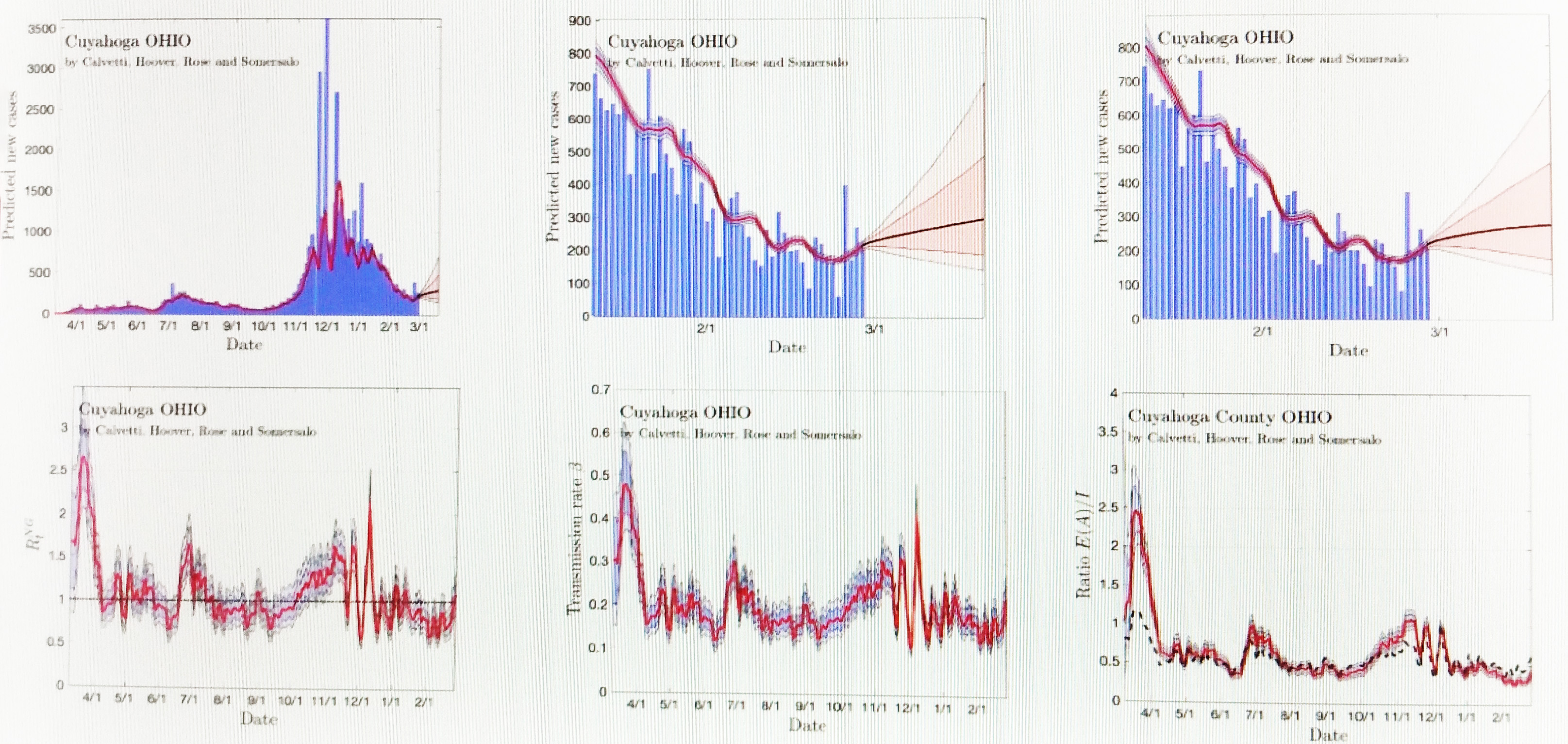
Calvetti began with a variation of the standard SEIR model that included “susceptible” \((S)\) “exposed” \((E)\), “asymptotic” \((A)\), “infected” (for patients with symptoms) \((I)\), “deceased” \((D)\), and “recovered” \((R)\) compartments. Because COVID-19 is presumably predominantly spread by unknowingly asymptomatic individuals (symptomatic cases are technically in quarantine), the asymptomatic component is particularly important. “The big question is, how do we track exposed, asymptomatic individuals?” Calvetti asked. It is difficult to truly separate asymptotic spreaders and estimate flow from the exposed to asymptomatic compartment. Therefore, Calvetti chose to merge these two compartments together into \(E(A) = E +A\) (see Figure 1).

Unless they succumb to the virus, all \(E(A)\) and \(I\) individuals eventually recover. For the purpose of her model, Calvetti assumed that recovered individuals are no longer susceptible. Model variables include transmission rate, recovery rate, the rate at which symptoms develop, death rate, and proportion of asymptomatic and symptomatic infectious individuals in circulation. Daily counts of new infections, deaths, and vaccinations comprise the model data, and data granularity occurs at the county level. Unfortunately, this data is susceptible to gaps, delays, and errors and is therefore quite messy. While Calvetti and her team can guess some of the parameters, there are others that they do not really know. “It would be foolish to fix them because there is a lot of behavior that is lumped into the parameters,” she said. It is thus better to keep the data flexible and think that the transmission rate is time dependent.

Calvetti then employed a Bayesian particle filtering framework to estimate both the model parameters and the size of the symptomatic and asymptomatic cohorts. Bayesian filtering methods are ideal for estimating the sequential time evolution of a dynamic model’s state vectors based on limited observations. Since the model’s variables—and the consequential spread of COVID-19—are continually evolving in time, Bayesian filtering is an effective choice. In a Bayesian framework, all unknown quantities become random variables, including the compartments’ size and the model parameters. Filtering techniques yielded a propagation model that Calvetti and her team evolved with numerical integration. They then combined this model with a multiplicative innovation model and defined the transition density.

After establishing the initial conditions, generating a cloud of initial state particles, introducing the basic reproduction number, and acknowledging the ratio of asymptomatic to symptomatic infections, Calvetti accounted for the effect of vaccines. To do so, she modeled vaccine distribution among the cohorts as a multinomial distribution and assumed that vaccinations proceed at prior week’s rate for the purpose of prediction.

Finally, Calvetti discussed her findings. She first displayed model predictions for a large county comprised of 1.5 million people (see Figure 2). She used model uncertainty to make predictions in three-week increments—now accounting for vaccine distribution—and has thus far been on target. Next she shared model predictions for a small county where the vaccine is not yet making much of a difference. She even analyzed Meade, S.D., in light of the Sturgis Motorcycle Rally in August 2020.

Calvetti concluded her presentation with a metapopulation model that examines the way in which people move between counties because of work. This model accounted for traffic flow in the context of both total freedom and travel restrictions between certain states. Calvetti specifically examined spatial patterns in the corridor between Pittsburgh, Pa.; Cleveland, Ohio; and Detroit, Mich. to identify automotive connections between cities. Over time, COVID-19 spread from metropolitan cities to rural areas. It runs the risk of surging back to the cities if mitigation efforts—like masks and social distancing—do not continue to complement reduced mobility; simply reducing traffic is not enough. Unfortunately, vaccines cannot replace mitigation just yet. But as long as preventative measure continue, public health sectors will not be overwhelmed.