Mixed-precision Computing: High Accuracy With Low Precision

Mixed-precision algorithms have launched an era in which efficiency and accuracy are no longer mutually exclusive. Mixed-precision arithmetic refers to the use of numbers of varying bit widths within a single computation or across different stages of an algorithm. Rather than rely entirely on high-precision formats like double (64-bit) precision, mixed-precision algorithms apply lower precisions—such as single (32-bit) or half (16-bit) precision—whenever possible, reserving higher precision only for critical steps. Doing so can drastically reduce memory requirements, improve performance, and lessen energy consumption on modern computer hardware without sacrificing accuracy or stability.

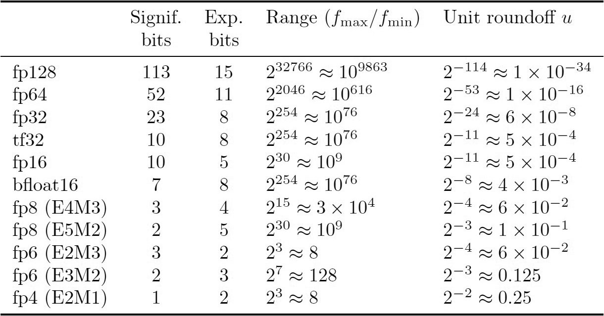
Computers have a finite number of bits for storage and computation. The industry standard—established in the 1980s by the Institute of Electrical and Electronics Engineers (IEEE)—is IEEE floating-point numbers. We can represent a base-2 floating-point number as \((-1)^{\textrm{sign}} \times 2^{\textrm{exponent-offset}} \times 1.\textrm{fraction},\) with \(1\) bit for the sign field and some number of bits for the exponent and fraction fields (see Figure 1). The number of exponent bits determines the range \(\pm [f_{\min}, f_{\max}]\) of representable numbers, and the number of fraction bits determines the unit roundoff \(u\): the relative precision with which numbers are stored. Virtually all current computers utilize this system.

Motivated by machine learning applications, modern graphics processing units (GPUs) now support multiple types of precisions—e.g., double, single, and half precision—as well as non-IEEE standard formats such as bfloat16, TensorFloat-32 (tf32), and variants of quarter (8-bit) precision. In fact, artificial intelligence (AI) applications have resulted in more devoted chip space for low-precision computations, which means that the potential speedups are superlinear in terms of the number of bits.

Mixed-precision hardware in supercomputers is a growing trend, with a steady increase in the TOP500 rankings of systems that use mixed-precision accelerators. Therefore, ignoring the availability of low-precision hardware during algorithm development is akin to leaving potential performance on the table. In today’s world, we must rethink our algorithms to determine when and where different precision formats can improve performance while still maintaining accuracy and stability. Of course, doing this in an effective, rigorous way involves numerous challenges.

Challenges of Low/Mixed Precision

The need for tight descriptive error bounds and adaptive approaches: When utilizing low and mixed precision, we need to ensure that computational errors remain controlled and predictable. Doing so necessitates the use of (mixed) finite-precision rounding error analysis to develop error bounds that provide guidance on precision configuration in different parts of the computation. For many relatively simple algorithms, such as direct solvers for dense linear systems, we can extend established techniques to accomplish this goal. But when dealing with complex, real-world applications, it is much harder to track the accumulation of rounding errors and their amplification of other errors throughout a large code base.

In any case, the obtained error bounds are data dependent according to problem dimension, conditioning, the norms of various involved quantities, and so forth. Since we often do not know these properties until runtime (and maybe not even then), it is frequently impossible to choose the correct precisions a priori. This limitation requires adaptive approaches that dynamically adjust precisions based on input and/or monitoring throughout the computation.

The (in)validity of error bounds for large-scale applications: Bounds on backward and forward errors typically only hold under certain constraints and often take forms like \(nu<1.\) In the context of low precision for large-scale computations, such constraints can be problematic. Here, the potentially large size of both \(n\) and \(u\) means that these constraints may not hold and error bounds that are derived in the traditional way might not be valid.

Interestingly, rounding error bounds are typically quite loose. As such, the algorithm output regularly satisfies the error bounds despite violation of the theorem constraints. This reality has motivated many researchers to rely on methods that derive tighter error bounds, e.g., via probabilistic rounding error analysis [3].

Working with a limited range: Most analyses of algorithm accuracy and stability assume that no overflow or underflow occurs. In the IEEE 754 standard, overflow and underflow mean that numerical values respectively become \(\pm\infty\) or \(0.\) While this assumption might be reasonable for double precision, overflow and underflow happen much more frequently in lower precisions.

We can address this challenge by developing procedures that avoid errors in the first place, such as a sophisticated scaling and/or shifting technique to “squeeze” matrix entries within a given range. The right scaling factors may not be obvious; in Gaussian elimination, for example, we should scale according to the pivot growth factor, which is often not immediately evident.

Another difficulty stems from the software engineering aspect. Users must carefully implement code to detect and resolve errors as they occur. While the detection of overflow is usually straightforward, recognizing underflow may be more difficult because it is not always clear whether a number should actually be \(0.\) In some cases, underflow is benign; in others, it can cause algorithms to fail due to loss of matrix properties like nonsingularity or positive definiteness.

When Mixed Precision Makes Sense

The use of mixed precision is natural in a number of common cases.

When a self-correction mechanism is available: The prototypical example of algorithms that have a natural self-correction mechanism is iterative refinement for the solution of linear systems. Given an initial approximate solution \(x_i\) to \(Ax=b,\) iterative refinement repeatedly evaluates the residual \(r_i=b-Ax_i,\) solves \(Ad_i=r_i,\) and constructs the next approximate solution \(x_{i+1}=x_i+d_i.\) A key point is that the solve for \(d_i\) need not be especially accurate; to guarantee convergence, it only has to make some forward progress. Therefore, we can often utilize lower precision in this part of the computation. Many other algorithms also have self-correction mechanisms, which are often characterized by inner-outer solve schemes [4, sections 5-8].

When finite-precision error is small compared to other sources of error: Real-world applications involve a variety of errors: (i) errors from modeling, discretization, and measurement; (ii) approximation errors from low-rank approximation, sparsification, and randomization; and (iii) truncation errors due to the use of stopping criteria in iterative methods. With all of these errors, we may wonder whether it is truly necessary to solve problems to such a high level of accuracy — we might be solving the wrong problem anyway.

To fully understand the lowest feasible level of precision, we must recognize the magnitude of the other errors at play; increasingly large errors mean that an increasingly low precision may be suitable. For example, consider the computation of a rank-\(k\) approximation of a matrix \(A.\) If we only want a very rough approximation where \(k\) is relatively small, then we can often perform the entire computation in lower precision. The difference between \(A\) and its low-rank approximation \(A_k\) could be the same order of magnitude regardless of precision type, since the error due to low-rank approximation will dominate.

When the computation naturally contains less sensitive subparts: Mixed precision is natural in computations that comprise subparts with intrinsically different sensitivity. In this case, a subpart’s sensitivity depends on the way in which a local error in the subpart affects the accuracy of the global computation. Such sensitivity may take different forms based on the application; a few concrete examples of things that can be stored in lower precision include elements of a matrix if their magnitudes are sufficiently small, singular vectors if their associated singular values are sufficiently small, and diagonal blocks if their condition numbers are sufficiently small. For all of these examples, the potential use of lower precision completely depends on the data. To leverage this potential, we must hence develop adaptive precision algorithms that dynamically select each subpart’s precision at runtime. And since the variations in sensitivity are often continuous, we can better adapt to the problem if more precision formats are available [4, section 14].

When low-precision hardware can efficiently emulate high precision: Motivated by deep learning applications, the computational power of current supercomputers comes almost entirely from GPU accelerators with specialized computing units—such as NVIDIA tensor cores—that are tailored for matrix multiplication in extremely low precision (e.g., 16- or even 8-, 6-, or 4-bit). 

While these precisions are very low, they are also very fast; for instance, 8-bit arithmetic is more than 100 times faster than 64-bit arithmetic on NVIDIA Blackwell GPUs. This speed has motivated a new class of mixed-precision algorithms that emulate high-precision matrix multiplication based on low-precision units. The main idea is to split the matrices into multiple “words” that are stored in lower precision. For example, we can represent an fp32 matrix (24 fraction bits) as the sum of three bfloat16 matrices (8 fraction bits each). We then reconstruct the result from the individual word products. The number of required products can span three to several dozen depending on the precisions in question, the emulation algorithm, and the dynamical range of the matrix elements [4, section 13].

When data transfers are the bottleneck: The volume of data transfers between processors or levels of the memory hierarchy strongly influences performance in many applications. Thus, a natural strategy to accelerate these memory-bound applications is to store the transferred data in lower precision. It is sometimes meaningful to decouple this lower storage precision from the compute precision, which remains high to preserve accuracy. In particular, the storage precision has no effect on rounding error accumulation. Decoupling the storage and compute precisions necessitates the development of memory accessors, which access the stored data in low precision and convert it to high precision for the purpose of computation. Besides reducing error accumulation, this type of approach does not require the storage precision to be a standard, hardware-supported arithmetic because it is not used in computations. We can therefore employ custom data formats—such as floating point with truncated fraction and/or exponent—that provide more flexibility when tuning the storage-accuracy tradeoff [1, section 4.3].

Impact on Applications

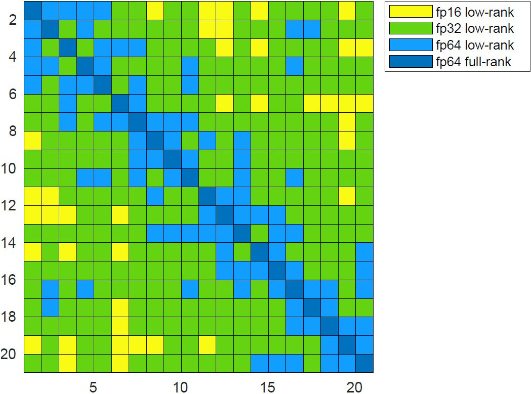
Figure 2 illustrates the mixed-precision opportunities that arise in the block low-rank approximation of a dense matrix. Specifically, off-diagonal blocks exhibit rapidly decaying singular values and are thus amenable to both low-rank truncation and reduced precision, all while preserving high accuracy relative to the entire matrix. Researchers have used this mixed-precision method in both dense and sparse direct solvers, resulting in significant storage and performance gains in climate and geoscience applications [2, 5]. For instance, the method led to a \(3\times\) reduction in storage requirements, allowing for the solution of a system with nearly 500 million unknowns — one of the largest real-world problems ever solved by a direct solver [5]. This is merely one example of the potential of mixed-precision algorithms, which users have successfully employed in many other application fields. 

Ultimately, we believe that a significant opportunity exists for a broad set of algorithms and scientific applications to benefit from the use of mixed precision. We end by asking readers to consider where they can potentially use less than the standard double precision to improve performance in their own computations.

References 
[1] Abdelfattah, A., Anzt, H., Boman, E.G., Carson, E., Cojean, T., Dongarra, J., … Yang, U.M. (2021). A survey of numerical linear algebra methods utilizing mixed-precision arithmetic. Int. J. High Perform. Comput. Appl., 35(4), 344-369.
[2] Abdulah, S., Cao, Q., Pei, Y., Bosilca, G., Dongarra, J., Genton, M.G., … Sun, Y. (2021). Accelerating geostatistical modeling and prediction with mixed-precision computations: A high-productivity approach with PaRSEC. IEEE Trans. Parallel Distrib. Syst., 33(4), 964-976.
[3] Higham, N.J., & Mary, T. (2019). A new approach to probabilistic rounding error analysis. SIAM J. Sci. Comput., 41(5), A2815-A2835.
[4] Higham, N.J., & Mary, T. (2022). Mixed precision algorithms in numerical linear algebra. Acta Numer., 31, 347-414.
[5] Operto, S., Amestoy, P., Aghamiry, H., Beller, S., Buttari, A., Combe, L., … Tournier, P.-H. (2023). Is 3D frequency-domain FWI of full-azimuth/long-offset OBN data feasible? The Gorgon data FWI case study. Lead. Edge, 42(3), 173-183.