Navier-Stokes Equations and Mimetic Operators

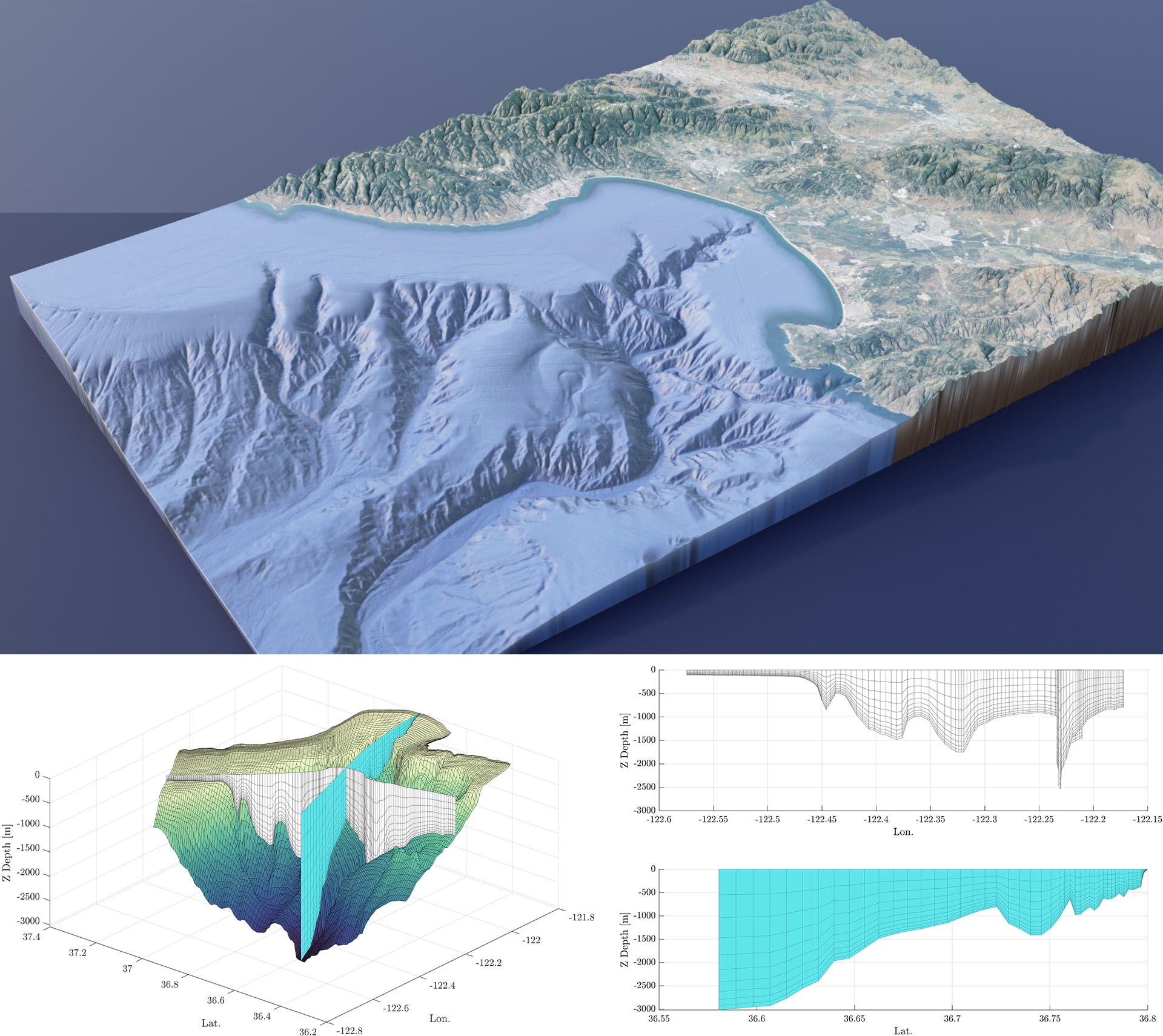
The Navier-Stokes (NS) equations are some of the most important equations in the physical sciences, and researchers routinely utilize a wide array of numerical methods to efficiently solve them. From a computational perspective, explicit finite differences are the simplest technique to implement; they are easy to parallelize and may be the fastest in terms of wall time, which makes them a popular choice for extensive geospheric simulations. Unfortunately, these benefits are nullified in the presence of a complex computational grid, such as in models of coastal canyons (see Figure 1). Scientists may instead use curvilinear coordinates—which are well suited for complicated areas because they are topologically equivalent to rectangles—to tackle these complex regions. However, additional difficulties arise for curvilinear coordinates in three dimensions. 

Because complicated equations often become cumbersome in arbitrary coordinate space, we seek to solve the NS equations in complex geometries while retaining the computational efficiency and ease of implementation of a finite difference method on a rectilinear grid. Luckily, using curvilinear coordinates to map a domain to a cube allows us to impose the boundary conditions on the computational grid, which is more straightforward than the same action in the physical domain.

We propose the use of mimetic difference methods to solve the NS equations in order to retain both speed and ease of implementation. These numerical schemes are based on mimetic difference operators: discrete analogs for the vector calculus operators of gradient and divergence that satisfy a discrete, extended version of Gauss’ divergence theorem. They are conservative, have a high order of accuracy on curvilinear grids, and remain close to the physics of the solution [1-4].

The Mimetic Operators Library Enhanced (MOLE)—which comes with C++ and MATLAB functions—provides the mimetic operators of divergence, gradient, Laplacian, and curl in one, two, and three dimensions with second-, fourth-, and sixth-order approximations. Given an appropriate three-dimensional (3D) grid that is defined by \(\textrm{X}\), \(\textrm{Y}\), and \(\textrm{Z}\), the creation of a second-order 3D curvilinear operator is as simple as D = div3Dcurv(2, X, Y, Z).

Navier-Stokes: Rescale and Transform

The incompressible non-dimensionalized NS equation that we are solving takes the following form:

\[\frac{\partial{\hat{\pmb{u}}}}{\partial t}+\hat{\pmb{u}} \cdot (\nabla \hat{\pmb{u}}) = -\frac{1}{\rho}\nabla \hat{p} + \frac{1}{Re}\nabla^2 \hat{\pmb{u}} + \frac{1}{Fr^2}\hat{S}. \tag1\]

We wish to solve this system of equations on a curvilinear grid; if we use the mimetic operators \(\tilde{\pmb{D}}\), \(\tilde{\pmb{G}}\), and \(\tilde{\pmb{L}}\), then doing so is equivalent to transforming the operators as

\[\frac{\partial\hat{\pmb{u}}}{\partial t} + \hat{\pmb{u}} \cdot (\tilde{\pmb{D}} \hat{\pmb{u}}) =  -\frac{1}{\rho}\tilde{\pmb{G}} \hat{p} + \frac{1}{Re}\tilde{\pmb{L}}\hat{\pmb{u}} + \frac{1}{Fr^2}\hat{S}. \tag2\]

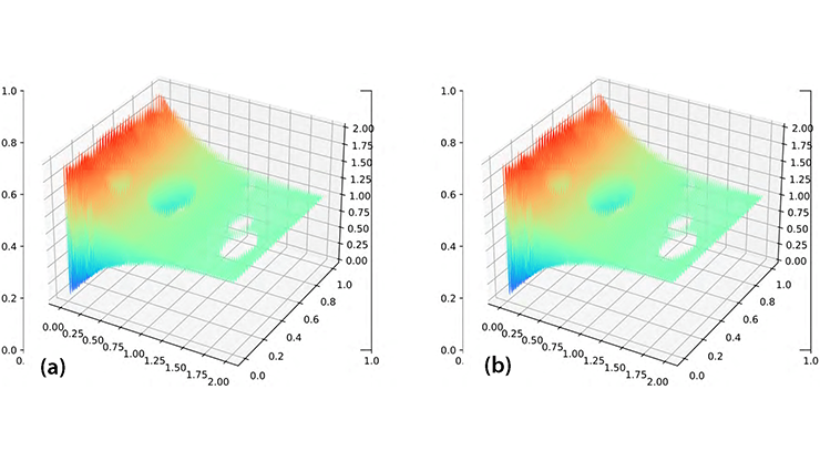
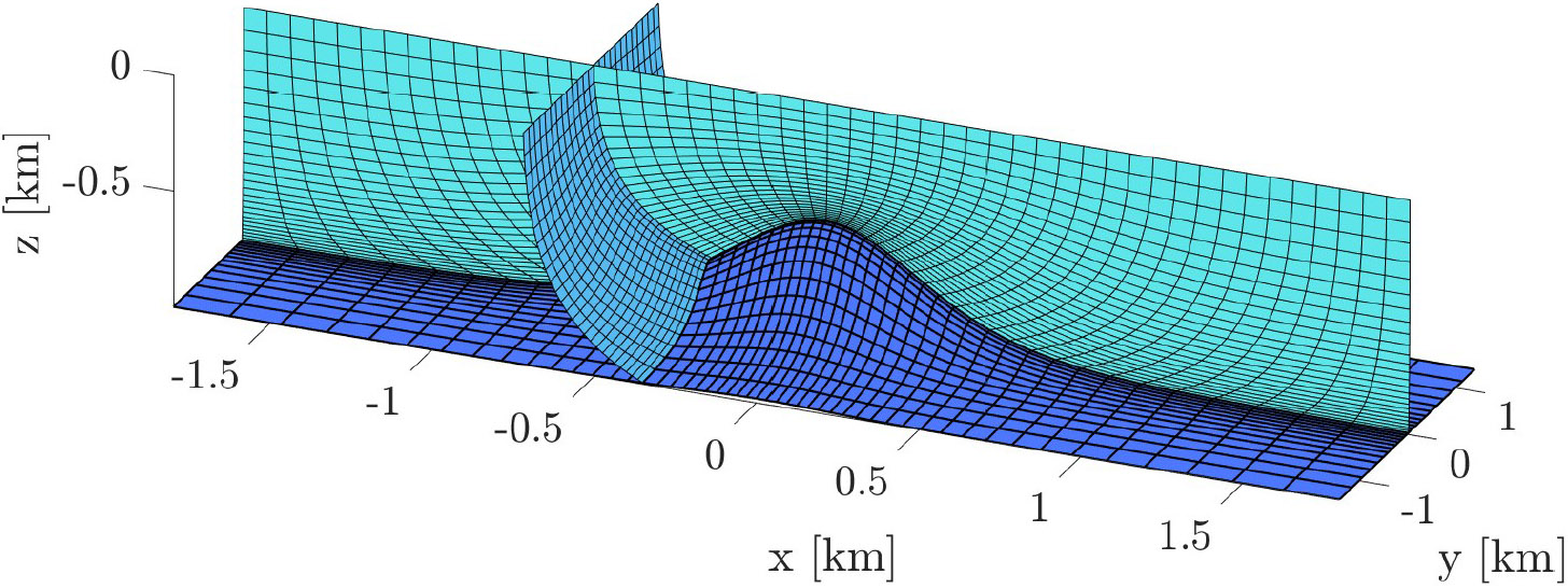
The code, which is entirely in C++, uses the MOLE C++ and Armadillo libraries to handle array building [6]; it relies on SuperLU for the solution of sparse systems [5]. By saving the decomposition of the left matrix, we can achieve a speedup that is 100 times greater than previous forms of this model. We tested the implementation in C++ on several iconic benchmark cases to assess the technique’s accuracy and verify the model’s behavior, ultimately determining the flow over a seamount via a curvilinear grid (see Figures 2 and 3).

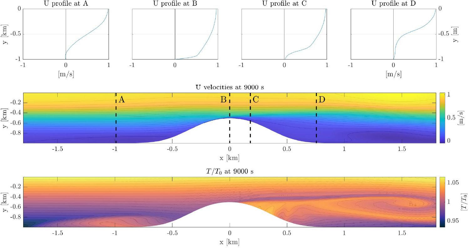
While the results are good, the required time for the curvilinear solution is orders of magnitude slower than the rectilinear case. The C++ code uses the curvilinear Laplacian \(\tilde{\pmb{L}}\) and estimated velocities \(\hat{u}\) to solve a system for pressure \(\tilde{\pmb{L}}p=\hat{u}\); it remains unclear why a sparse system solver has so much trouble with the curvilinear matrix. This obstruction has stifled further use of the method, as SuperLU struggles to extract features from the matrix. With roughly three times as many nonzero entries, the calculation takes 100 times longer, which negates all previous time savings. Perhaps the matrix’s non-banded nature is to blame, as the curvilinear Laplacian matrix is not positive definite, symmetric, or banded. We are currently searching for a way to more quickly solve this system in order to tackle increasingly complex, realistic problems in geophysical flows in a computationally efficient manner, thus enabling realistic and usable predictions.

Jared Brzenski delivered a minisymposium presentation on this research at the 10th International Congress on Industrial and Applied Mathematics (ICIAM 2023), which took place in Tokyo, Japan, last year. He received funding to attend ICIAM 2023 through a SIAM Travel Award that was supported by U.S. National Science Foundation grant DMS-2233032. To learn more about SIAM Travel Awards and submit an application, visit the online page.

References
[1] Brzenski, J., & Castillo, J.E. (2023). Solving Navier-Stokes with mimetic operators. Comput. Fluids, 254, 105817.
[2] Castillo, J.E, Hyman, J.M., Shashkov, M.J., & Steinberg, S. (1995). The sensitivity and accuracy of fourth order finite-difference schemes on non-uniform grids in one dimension. Comput. Math. Appl., 30(8), 41-55.
[3] Castillo, J.E., & Miranda, G.F. (2013). Mimetic discretization methods. New York, NY: CRC Press.
[4] Corbino, J., & Castillo, J.E. (2020). High-order mimetic finite-difference operators satisfying the extended Gauss divergence theorem. J. Comput. Appl. Math., 364, 112326.
[5] Li, X.S. (2005). An overview of SuperLU: Algorithms, implementation, and user interface. ACM Trans. Math. Softw., 31(3), 302-325.
[6] Sanderson, C., & Curtin, R. (2020). An adaptive solver for systems of linear equations. In 2020 14th International Conference on Signal Processing and Communication Systems (ICSPCS). Institute of Electrical and Electronics Engineers.