Newtonian Dynamics = “Spring Theory”

A simple but illuminating equivalence exists between Newtonian mechanics of a particle and the statics of Hookean springs. In light of this equivalence, some basic facts of Hamiltonian mechanics become truly transparent. One can see, with very few formulas, why energy is conserved in Hamiltonian systems and why these systems preserve Poincaré’s integral invariants, among other things. Here is a brief sketch of this equivalence; more details can be found in [1].

We look at a point mass \(m\) with potential energy \(P=P(x) , x\in  {\mathbb R}  ^n\) in some conservative force field. Hamilton’s principle in this setting says that the motions \(x(t)\) are stationary functions of the action

\[ \int_{0}^T \biggl (\frac{m\dot x^2}{2} - P(x) \biggl) dt \equiv \int_{0}^{T} (K-P)dt   \qquad (1)\]

with fixed ends \((0,x_0)\) and \((T, x_T)\) in the time-space \((t,x)\).

Generations of students of the subject have been bothered by the depressing lack of a physical interpretation of the difference \(K-P\). Einstein made an absolutely striking observation that (1) is the first significant term in the relativistic expression \(\int E\,dt^\ast,\) where \(t^\ast\) is the particle’s proper time and \(E\) is the energy; so, (1) does have an independent meaning – a relativistic one. Setting this gem aside, however, I would like to stick to classical mechanics.

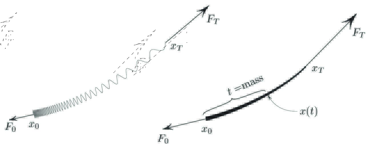
The action (1)—which comes from dynamics—admits a static interpretation. As an Archemedian thought experiment, let’s hang an idealized spring by two ends (see Figure 1). Consider the child’s toy “slinky,” which we treat as a one-dimensional object, perhaps thinking of it alternatively as a heavy rubber band that stretches non-uniformly, as shown in the same figure. There is no resistance to bending, and our spring satisfies linear Hooke’s law. The spring has mass, and we denote Hooke’s constant of the unit mass of the spring by \(m,\) suggestively.¹

We parametrize the position \(x(t)\) of the spring’s particle by the mass \(t\) between the particle and the spring’s end, as seen in Figure 1. The spring’s total potential energy then turns out to be

\[ \int_{0}^{T}   \biggl( \frac{m\dot x ^2 }{2} + U(x) \biggl)  \,dt , \qquad (2) \]

where \(U(x)\) is the potential energy of a unit mass; the term \(\frac{m\dot x ^2 }{2}\) is the stretching energy per unit mass.

Now (2) coincides with (1) if  \(P= -U.\) We endowed the dynamic action (1) with a static meaning: the action (1) is the potential energy of a slinky placed in the force field with potential \(−P.\) Since I used no special features of the gravitational field, this statement applies to any potential \(P.\)

And so the Newtonian dynamics is equivalent to statics of springs. A table of equivalence can be found on page 45 of [1], and lists static equivalents of velocity, momentum, etc.

Here are some examples and consequences of the aforementioned equivalence:

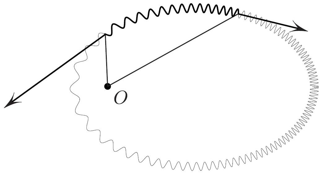
1. Connect the two ends of the slinky, making a loop, and place it in the repelling Coulomb field with potential \(U= \frac{1}{r}\) in \({\mathbb R} ^3\) (see Figure 2). What are the possible equilibrium shapes of the loop? This is a static equivalent of Kepler’s problem (in the potential \(−U)\). We conclude that the equilibria are ellipses (assuming that the mass  \(T\) of the spring is finite, which excludes parabolas and hyperbolas).

2. In the preceding example, what is the static equivalent of the conservation of angular momentum? It is the following: for any arc of the spring in the equilibrium in a central potential, the torques of the two tension forces exerted on the ends of the arc by the rest of the spring cancel each other out (torques are computed relative to the origin). Conservation of the angular momentum is thus a consequence of Newton’s first law in its rotational version: zero angular acceleration means zero torque.

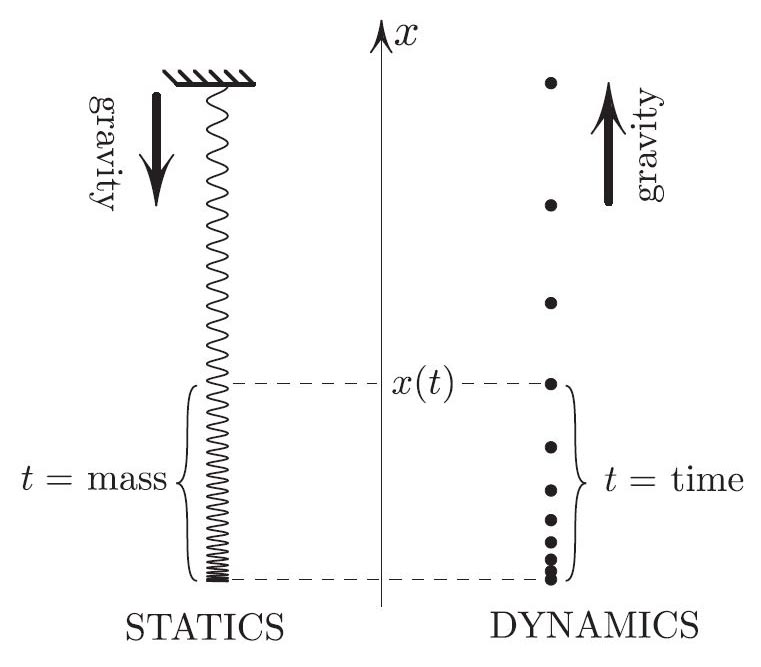
3. Conservation of total energy \(K+P\) in dynamics has a static counterpart. What is it? By asking this question I discovered something I hadn’t realized before but is obvious in retrospect: the difference \(K-U\) between the energy densities (per unit mass) of stretching and of “elevation” is constant along the spring in equilibrium. As an example, consider the hanging spring in Figure 3. The higher the loop, the more it is stretched, i.e. both energy densities increase with height – interestingly, by the same amount! This remark applies to any potential field, for instance to the Coulomb field of the previous example.

4. This is a (literally) hand-waving explanation of Poincaré’s integral invariance. Imagine holding both ends of the spring in Figure 1 and moving the two hands cyclically and slowly, so as not to excite any vibrations. In doing so we perform zero net work:

\[ \oint F_0 \cdot dx_0 + \oint F_T \cdot dx_T=0, \qquad (3) \]

with \(F_0 , F_T\) denoting the forces we exert. Putting this formula through the statics-dynamics dictionary leads to

\[ \oint_{C_0} p_0 \cdot dx_0 = \oint_{C_T} p_T \cdot dx_T, \qquad (4) \]

where \(p= m \dot x\) is the momentum, \(C_0\) is a curve of initial data in phase space \(\{(x, \dot x )\}\), and \(C_T\) is the image of this curve under the phase flow after time \(T\). Therefore, the Poincaré integral invariance follows from the general principle that a perpetual motion machine cannot work. Note that it was not even necessary to write the Hamiltonian equations of motion to obtain (4).

5. A quick derivation of the Euler-Lagrange equation for (1), bypassing the (more general) method of Euler and Lagrange, is to observe that one can interpret the minimizer of (1) as a minimizer of the potential energy of a spring in the field with potential \(-P\). But a spring in such an energy-minimizing state is in equilibrium, and thus the sum of forces on each infinitesimal element vanishes. There are three of these forces: two tensions on the ends, \(m \dot x(t+dt)\) and \(-m\dot x (t)\), and the force due to the ambient field, \(P ^\prime  (x(t))dt+ O( dt^2)\). Dividing the sum of all these by \(dt\) and setting \(dt \rightarrow 0\) gives \(m\ddot x +P ^\prime (x)=0\). We derived the Euler–Lagrange equation for (1) from Newton’s first law.

¹ More details on all of this can be found in [1].

References

[1] Levi, M. (2014, March). Classical Mechanics with Calculus of Variations and Optimal Control: an Intuitive Introduction. AMS, 42-49 & 274-280.