Numerics for Stochastics

The following is a brief contribution from the authors of An Introduction to the Numerical Simulation of Stochastic Differential Equations, which was published by SIAM in 2021. This book describes the numerical solution of stochastic differential equations and is suitable for a broad audience that ranges from undergraduate students to established researchers. Computational examples illustrate key ideas, computer code supplements each chapter, and 150 exercises and 40 programming projects provide further opportunities for readers to explore the material.

The authors also share a short excerpt about the Fokker-Planck equation from chapter 14, titled “Steady States.” It has been abridged and edited for clarity.

An Introduction to the Numerical Simulation of Stochastic Differential Equations is a lively, accessible presentation of the numerical solution of stochastic differential equations (SDEs). We kept the prerequisites to a minimum to ensure that the topic is accessible to the widest conceivable readership, and only assumed a competence in algebra and first-year undergraduate calculus. A major motivation for this book was the sustained citation level of a 2001 article on the subject that appeared in the “Education” section of SIAM Review [3]. Based on that impactful publication and ensuing discussions with colleagues, we identified a definite need for a self-contained, elementary text that conveys the fundamentals as succinctly as possible. Our book follows the style of the original article [3] and offers a myriad of computational examples and illustrative figures to support the concepts.

Because the field of numerical SDEs is relatively new but rapidly expanding, we were able to include novel material on modern topics that did not appear outside of research articles and monographs at the time of publication, including the following areas:

• Failure of the standard Euler-Maruyama method to converge for a simple nonlinear SDE
• Asymptotic and mean-square stability for numerical SDEs
• Mean exit times
• Exotic options in mathematical finance
• Steady state behavior
• Multilevel Monte Carlo methods
• SDEs with jumps
• SDE models in the social sciences
• Modeling with colored noise
• Pitfalls in the approximation of double stochastic integrals
• Stochastic modeling and simulation regimes in chemical kinetics.

Many aspects of numerical SDEs can be confusing and sometimes raise questions that are as philosophical as they are mathematical. Within the limitations of accessibility, we aimed to clearly explain the issues that surround strong versus weak solutions and convergence, Itô versus Stratonovich calculus, mean-square versus asymptotic stability, and the thermodynamic limit.

In our experience, the best way to understand an algorithm is to experiment with a suitable computer program. For this reason, each chapter of An Introduction to the Numerical Simulation of Stochastic Differential Equations concludes with a full walkthrough of a “Program of the Chapter” that explores a key topic.

The following excerpt about the computation of long-time trajectories combines selected parts of chapter 14 on “Steady States.” This topic continues to be an important research area, not least because of its connections to modern algorithms in statistical sampling and machine learning.

Meet the Fokker-Planck Equation

For a deterministic ordinary differential equation (ODE) \(\textrm{d}x(t)/\textrm{d}t = f(x(t))\), any point \(x^\star\) such that \(f(x^\star) = 0\) is a steady state. A solution that begins at a steady state will remain there because the derivative will always be \(0\). And if \(x^\star\) is a locally attractive steady state, then initial conditions that are sufficiently close to \(x^\star\) will produce solutions for which \(x(t) \to x^\star\) as \(t \to \infty\). If all solutions approach the fixed point, it is said to be globally attractive.

These concepts extend to SDEs. In particular, any point \(x^\star\) such that \(f(x^\star) = g(x^\star) = 0\) is a fixed point of the SDE

\[\textrm{d}X(t) = f( X(t)) \textrm{d} t + g ( X(t)) \textrm{d} W(t).\]

However, a more general scenario is also possible. Because \(X(t)\) is a random variable at each time \(t\), we can think of it as being characterized by a density function \(p(x,t)\); for each time \(t\), the integral \(\int_{a}^{b} p(x,t)\,\textrm{d}x\) gives the probability that \(a \le X(t) \le b\). Since \(p(x,t)\) is a function of two variables, it is reasonable to imagine that it satisfies a partial differential equation (PDE). This is indeed the case under appropriate conditions, and the relevant PDE takes the form of the Fokker-Planck or Kolmogorov forward PDE:

\[\frac{ \partial }{\partial t} p(x,t) + \frac{ \partial }{\partial x} ( f(x) p(x,t)) - \frac{1}{2} \frac{ \partial^2 }{\partial x^2} (g(x)^2  p(x,t)) = 0. \tag1\]

If the solution approaches a time-invariant limit as \(t\to \infty\), we can logically consider a steady state density function \(p(x)\) that stems from setting the time derivative in \((1)\) to \(0\). Doing so leads to the ODE

\[\frac{\textrm{d}}{\textrm{d} x} (f(x)  p(x)) - \frac{1}{2} \frac{\textrm{d}^2}{\textrm{d} x^2} (g(x)^2  p(x)) = 0. \tag2\]

As an example, consider the Ornstein-Uhlenbeck process wherein \(f(x) = -\lambda x\), \(g(x) = \sigma\), and \(\lambda > 0\). The steady Fokker-Planck equation in \((2)\) becomes

\[-\lambda \frac{\textrm{d}}{\textrm{d}x} (xp(x)) - \tfrac{1}{2} \sigma ^2 \frac{\textrm{d}^2}{\textrm{d} x^2}p(x) = 0. \tag3\]

We find that the only solution to this ODE that corresponds to a density function over \(-\infty < x < \infty\) is

\[p(x) = \frac{1}{\sqrt{2\pi\sigma^2 /(2 \lambda)} }\textrm{e}^{- x^2/(2 \sigma^2/(2 \lambda))}, \tag4\]

i.e., the density of a \(N(0,\sigma^2/(2 \lambda))\) random variable. All solutions approach this steady state. This finding is consistent with the properties

\[\mathbb{E} [ X(t)] \to 0 \quad \textrm{as} \quad  t \to \infty\]

and

\[\mathbb{E} [ X(t)^2]  \to  \frac{ \sigma^2}{2 \lambda} \quad \textrm{as} \quad t \to \infty; \tag5\]

the latter of these follows from Itô’s formula.

Computing to a Steady State 

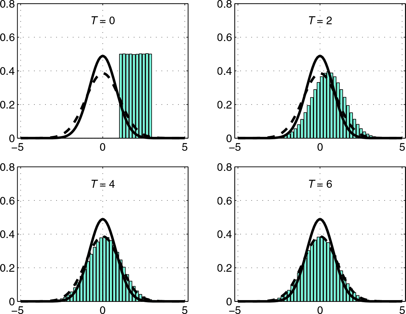
In Figure 1, we take \(\lambda = 0.75\), \(\sigma = 1\), and \(X(0)\) uniformly over \((1,3)\) in the Ornstein-Uhlenbeck process. We then apply the Euler-Maruyama method with step size \(\Delta t = 1\) and generate histograms for the time \(T\) solutions that arise from \(10^6\) independent paths. We deliberately chose a large \(\Delta t\) to emphasize the fact that the exact and Euler-Maruyama steady states are not equal. Figure 1 depicts the initial data \(X_0\) and provides computations for times \(T=2\), \(T=4\), and \(T=6\). The solid and dashed curves respectively represent analytical expressions for the exact and Euler-Maruyama steady state densities of this simple SDE.

Additional Notes

Algorithms that time-step toward the steady state of a differential equation are intimately connected to algorithms that iterate toward the solution of an optimization problem. In particular, we can utilize an SDE viewpoint [7] to interpret the stochastic gradient method, which is widely used in the field of deep learning to train artificial neural networks [2].

Time-stepping to a steady state is also a useful way to generate samples from a given distribution. Suppose that we wish to sample from a random variable with density \(p(x) = C\rho(x)\), where we do not need to explicitly specify the normalizing constant \(C\) that makes \(\int_{-\infty}^{\infty} p(x) = 1\). First, we write \(\rho(x) = \textrm{e}^{-V(x)}\) for some function \(V(\cdot)\). We see that the SDE with \(f(x) = -V'(x)\) and \(g(x) =\sqrt{2}\) has the appropriate invariant measure. We may hence compute an approximate sample by following the SDE’s path for a sufficiently long time. 

In the Markov chain Monte Carlo setting, researchers have combined this idea with a Metropolis-Hastings-style acceptance/rejection step [6] to produce a method that is now called the Metropolis-adjusted Langevin algorithm [1, 4, 5]. This algorithm is particularly effective for multidimensional distributions. When the SDE is ergodic, averaging over a long time period is equivalent to averaging over all paths. Therefore, to compute \(\mathbb{E} [\phi(X^\star)]\)—where the random variable \(X^\star\) represents the stationary distribution—it is reasonable to truncate \(T\) at a suitably large value and compute an approximation to \(\lim_{T \to \infty} T^{-1} \int_{0}^{T} \phi(X(t))\textrm{d}t\) for a single path.

Enjoy this passage? Visit the SIAM Bookstore to learn more about An Introduction to the Numerical Simulation of Stochastic Differential Equations and browse other SIAM titles. Additionally, two book reviews of this text have published in SIAM Review; Guenther Leobacher of the University of Graz offered his impressions in the December 2023 issue (Vol. 65, Issue 4), and Minh-Binh Tran of Texas A&M University shared his thoughts in the March 2024 issue (Vol. 66, Issue 1). 

References 
[1] Bou-Rabee, N., & Hairer, M. (2013). Nonasymptotic mixing of the MALA algorithm. IMA J. Numer. Anal., 33(1), 80-110.
[2] Higham, C.F., & Higham, D.J. (2019). Deep learning: An introduction for applied mathematicians. SIAM Rev., 61(4), 860-891.
[3] Higham, D.J. (2001). An algorithmic introduction to numerical simulation of stochastic differential equations. SIAM Rev., 43(3), 525-546.
[4] Kuntz, J., Ottobre, M., & Stuart, A.M. (2018). Non-stationary phase of the MALA algorithm. Stoch. PDE: Anal. Comp., 6(3), 446-499.
[5] Pereyra, M., Schniter, P., Chouzenoux, É., Pesquet, J.-C., Tourneret, J.-Y., Hero, A.O., & McLaughlin, S. (2016). A survey of stochastic simulation and optimization methods in signal processing. IEEE J. Sel. Top. Signal Process., 10(2), 224-241.
[6] Roberts, G.O., & Tweedie, R.L. (1996). Exponential convergence of Langevin distributions and their discrete approximations. Bernoulli, 2(4), 341-363.
[7] Sirignano, J., & Spiliopoulos, K. (2017). Stochastic gradient descent in continuous time. SIAM J. Financial Math., 8(1), 933-961.