Predicting the Shape of Evolutionary Trees
The following is a short excerpt from Phylogeny: Discrete and Random Processes in Evolution by Mike Steel, which was published by SIAM in 2016. This text comes from chapter three, “Tree Shape and Random Discrete Phylogenies,” and is modified slightly for clarity.
This excerpt is the first installment of a new SIAM News feature called “From the SIAM Bookshelf,” which will periodically spotlight SIAM texts in areas of wide appeal to the greater applied mathematics and computational science community.
The Shape of Evolving Trees
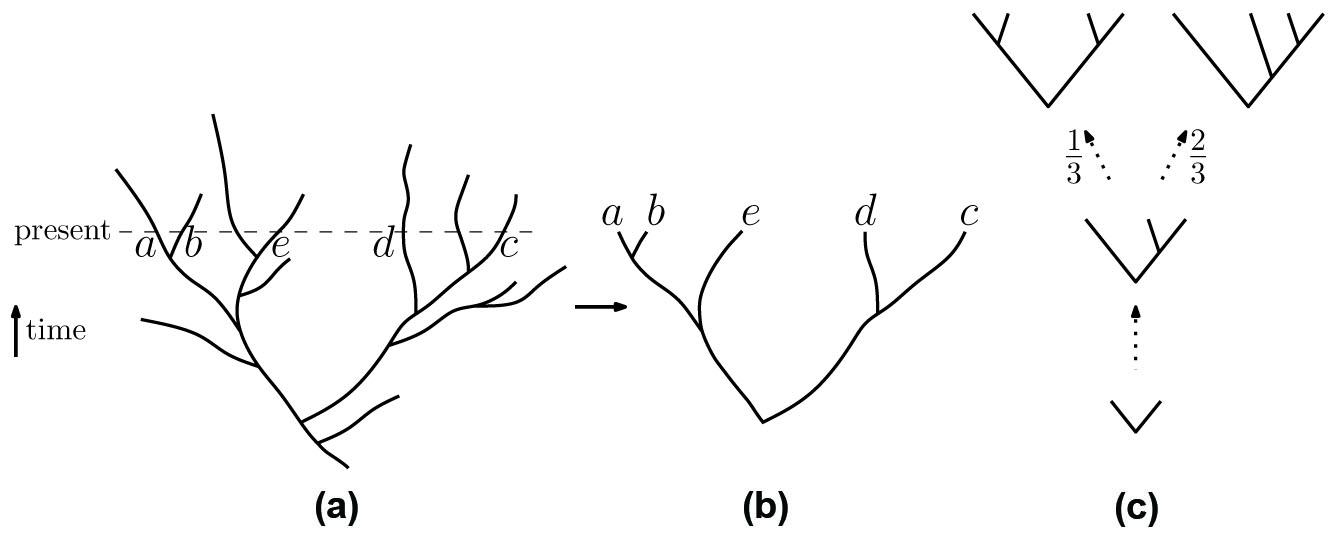
[Extinction has] played a major role in the history of life; after all, most species are extinct.1 Suppose we sample some subset \(X\) of species that are present today (species \(a\)-\(e\) in Figure 1a) and then consider the minimal tree linking these species. This results in the so-called “reconstructed tree” illustrated in Figure 1b. Let us view this as a rooted phylogenetic \(X\)-tree (ignoring the length of the edges). It turns out that under very general assumptions concerning the speciation-extinction process, many models predict an identical and simple discrete probability distribution on \(RB(X)\). Moreover, this discrete probability distribution can be easily described and is called the Yule-Harding (YH) model (or distribution).
To obtain a binary tree shape under the YH model, we start with a tree shape on two leaves and sequentially attach leaves, attaching a new leaf at each step to one of the leaf edges chosen uniformly at random from the tree constructed so far. For example, the probabilities of generating the fork and caterpillar tree shapes are \(\frac13\) and \(\frac23\) respectively, since from the (unique) tree shape on three leaves, we can attach a new leaf to exactly one of the three leaf edges to obtain a fork tree shape, or to any two of these leaf edges to obtain a caterpillar tree shape (see Figure 1c).

Once we have built up a tree with \(n\) leaves in this way, we obtain a random tree shape on \(n\) leaves and can now label the leaves of this tree shape according to a permutation on \(\{1,2, \ldots, n\}\), chosen uniformly at random. This is the YH probability distribution on \(RB(n)\).
We now explain how to compute the probability of a YH tree shape and that of any rooted phylogenetic tree with this shape. First, let us grow a tree under the YH process until it has \(n\) leaves, and then randomly select one of the two subtrees incident with the root (say, the “left-hand one” since the orientation in the plane plays no role) and let \(Z_n\) denote the number of leaves in this tree. Remarkably, \(Z_n\) has a completely flat distribution.
Lemma 1. \(Z_n\) has a uniform distribution between \(1\) and \(n-1\), so
\[\mathbb{P}(Z_n = i) = \frac{1}{n-1}, \mbox{ for } i = 1, \ldots, n-1.\]
Proof: The random process \(Z_1, Z_2, \ldots\) can be exactly described as a special case of a classical process in probability called Pólya’s urn. This consists of an urn that initially has \(a\) blue balls and \(b\) red balls. At each step, a ball is sampled uniformly at random and returned to the urn along with another ball of the same color. In our setting, \(a=b=1\) and “blue” corresponds to the left-hand subtree and “red” to the right-hand subtree in the YH tree. At each step, the uniform process of leaf attachment ensures that \(Z_n\) has exactly the same probability distribution as the number of blue balls in the urn after \(n-2\) steps. It is well known, and easily shown by induction, that in Pólya’s urn with \(a=b=1\), the proportion of blue balls has a uniform distribution.
Lemma 1 provides the key to computing the YH probability of a tree.
Proposition 1. For any particular tree \(T \in RB(n)\), the probability \(\mathbb{P}_{\rm YH}(T)\) of generating \(T\) under the YH model is given by
\[\mathbb{P}_{\rm YH}(T) = \frac{2^{n-1}}{n!\prod_{v \in \overset{\circ}{V}(T)} \lambda_v},\]
where \(\overset{\circ}{V}(T) \) is the set of interior vertices of \(T\) and \(\lambda_v\) is number of leaves of \(T\) that are descendants of \(v\), minus \(1\).

Proof: Suppose that the two maximal subtrees \(T_1\) and \(T_2\) of \(T\) are of size \(k\) and \(n-k\), where we may assume that \(2k \leq n\). By Lemma 1, the probability of such a size distribution is \(2/(n-1)\) if \(2k<n\) and \(1/(n-1)\) if \(2k=n\). Conditional on this division, the number of ways to select leaf sets for \(T_1\) and \(T_2\) that partition \([n]\) is \(\binom{n}{k}\) when \(2k<n\) and \(\frac{1}{2}\binom{n}{k}\) when \(2k=n\) (the factor of \(\frac{1}{2}\) recognizes that the order of \(T_1\) and \(T_2\) is interchangeable in \(T\) when they have the same number of leaves). By the Markovian nature of the YH process, each of these two subtrees also follows the YH distribution. This leads to the recursion
\[\mathbb{P}_{\rm YH}(T) = \frac{2}{n-1} \binom{n}{k}^{-1} \mathbb{P}_{\rm YH}(T_1)\mathbb{P}_{\rm YH}(T_2),\]
from which Proposition 1 now follows by induction.
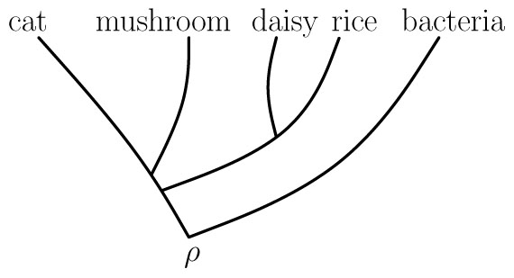
To illustrate Proposition 1, consider the tree in Figure 2. Then we have \(\mathbb{P}_{\rm YH}(T) = \frac{2^4}{5!\times 4\times 3\times 1^2}=\frac{1}{90}\), while the tree in Figure 1b gives \(\mathbb{P}_{\rm YH}(T) =\frac{1}{60}\).
Exercise: Find a general formula for the probability that a random tree \(\mathscr{T}\) in \(RB(n)\) generated by the YH model has the shape of a rooted caterpillar tree. What is the probability that \(\mathscr{T}=T\) for a particular caterpillar tree \(T \in RB(n)\)?
Curiously, a quite different process that arises in population genetics, and which proceeds backward in time (rather than forward, as in Figure 1c), also leads to the YH distribution when we ignore the length of the edges and the associated ranking of interior vertices. This is the celebrated coalescent process most usually associated with Sir John Kingman and developed in the early 1980s. As a discrete process, the coalescent starts with the set \(X\) and selects uniformly at random a pair of elements to join (these form the “cherry” of the tree that is closest to the leaves). These two leaves are then regarded as a single element in a set of size \(|X|-1\), and the process is repeated. This discrete coalescent process generates a ranked binary phylogeny, which is often referred to as a labeled history. This consists of a pair \((T, r)\), where \(T \in RB(X)\) and \(r\) is a ranking of the interior vertices of \(T\) — that is, a bijective function \(r: \overset{\circ}{V}(T) \rightarrow \{-1, -2, \ldots, -(n-1)\}\) with the property that if \(u\) is a descendant of \(v\), then \(r(u)>r(v)\) \((\)thus the root is the vertex assigned an \(r\) value of \(-(n-1))\). The function \(r\) describes the order in which the coalescent events occur, so the first cherry to form in the process has rank \(-1\), for instance.
1 It is estimated that current plant and animal diversity preserves at most one to two percent of the species that have existed over the past 600 million years.
Enjoy this passage? Visit the SIAM bookstore to learn more about Phylogeny: Discrete and Random Processes in Evolution and browse other SIAM titles.
Stay Up-to-Date with Email Alerts
Sign up for our monthly newsletter and emails about other topics of your choosing.


