Problem Solving With Multiple Solution Methods

Many problems in mathematics, science, and engineering can be solved in multiple ways — some of which require more time and resources than others. This decision is especially weighty for problem solvers who do not necessarily know the best path forward and have a finite window to complete the task at hand, such as undergraduate students taking an exam, Ph.D. candidates conducting research, or project managers deciding on an optimal strategy. Here, we aim to understand the process by which individuals address problems with several solution paths and ultimately prescribe strategies to improve and optimize this methodology.

A variety of existing studies have investigated the nature of problem solving. For example, a 2015 paper examined the spectrum between closed, well-defined problems with only one solution path and open, ill-defined problems with many possible approaches [1]. Another line of work seeks to understand students’ use of estimation—a quick tool that yields useful approximations prior to time-consuming analyses—to solve engineering problems [3, 4]. These studies provided background context for our own investigation. 

Problem Solving Experiment

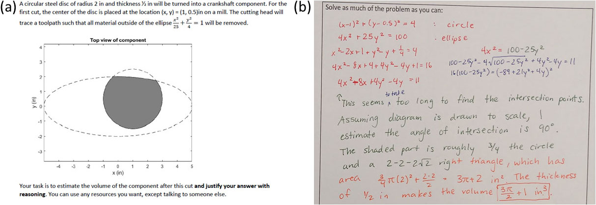
To explore the range of potential problem-solving approaches and their relative effectiveness, we conducted an educational experiment in which we presented a problem with several possible solution paths to 72 undergraduate and graduate students at the Massachusetts Institute of Technology (see Figure 1). Participants had five minutes to brainstorm and 10 minutes to solve as much of the problem as they could. They wrote their solutions on paper sheets and switched pen colors every two minutes so that we could track their progress over time. We analyzed their solutions in detail, sorting them based on approach and estimating the amount of time spent on each technique. 

Several trends emerged. First, the majority of students who failed to solve the problem simply did not finish within the time limit; mathematical errors or incorrect but complete solutions were uncommon. Second, students who used shorter, simpler methods were more likely to correctly solve the problem. In approximate order of increasing complexity, the solution methods included visual estimation, geometric approximation, computer-aided design, Monte Carlo methods, and integration. Third, students who attempted several different solution methods tended to solve the problem more often, but the number of students who implemented more than one method was small compared to the overall number of participants. This resulting data served as the basis for our model and helped us define key metrics to better understand problem solving with multiple solution methods.

Modeling, Analytic Solutions, and Optima

We used the observed trends to formulate a model for student outcomes [2]. Time is modeled continuously, and the simulated student must solve the problem within a time limit \(t_f\). At \(t=0\), the participant starts on one of \(n\) possible solution methods, selected with equal probability. These methods have solve times of \(t_1, t_2, \dots, t_n\); if the participant remains on a single method for at least as long as its solve time, they successfully solve the problem. The student switches methods as Poisson arrivals with a frequency of \(\lambda\), and the solve probability \(P_{\textrm{solve}}\) is a function of the switching frequency \(\lambda\). The problem solver’s goal is to maximize \(P_{\textrm{solve}}\) by varying \(\lambda\).

This model has two important assumptions. First, the problem solver does not necessarily know which solution method will be easiest or take the least amount of time (otherwise, the optimal solution path would be obvious). Second, there is a penalty for switching methods, as the problem solver loses all progress on their previous method.

We are able to derive \(P_{\textrm{solve}}(\lambda)\) for \(n=2\) solution methods in the case where the first method has a solve time of \(t_1 \le t_f\) and the second method has a solve time of \(t_2 > t_f\). We can analyze the probability of solving the problem for a fixed number of transitions \(B\), then sum the probabilities according to the likelihood of each case:

\[P_{\textrm{solve}}(\lambda) = \sum_{B = 0}^\infty{\frac{(\lambda t_f)^B e^{-\lambda t_f}}{B!}}P_{\textrm{solve}|B}(t_1^*).\]

Here, \(P_{\textrm{solve}|B}(t_1^*)\) is the probability of solving the problem—given fixed \(B\)—as a function of the first method’s nondimensionalized solve time \(t_1^* = \frac{t_1}{t_f}\). We can further express this idea as

\[P_{\textrm{solve}|B} = \begin{cases} p\left(B,\frac{B+1}2\right) & \text{if $B$ is odd}\\ \frac12{\left(p\left(B,\frac{B}2\right) + p\left(B,\frac{B}2+1\right)\right)} & \text{if $B$ is even},  \end{cases}\]

where

\[p(B,C) = \begin{cases} \binom{C}{1}(1-t_1^*)^B & \text{if } t_1^* \geq \frac12 \\ \binom{C}{1}(1-t_1^*)^B - \binom{C}{2}(1-2t_1^*)^B& \text{if } \frac13 \leq t_1^* < \frac12 \\ \binom{C}{1}(1-t_1^*)^B - \binom{C}{2}(1-2t_1^*)^B + \binom{C}{3}(1-3t_1^*)^B& \text{if } \frac14 \leq t_1^* < \frac13 \\ \vdots & \\ \binom{C}{1}(1-t_1^*)^B - \binom{C}{2}(1-2t_1^*)^B + \dots + \binom{C}{C}(-1)^{C+1}(1-Ct_1^*)^B & \text{if } t_1^* < \frac1C. \end{cases}\]

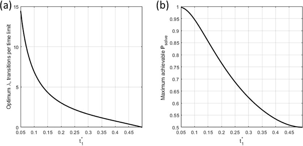
Using this analytic expression, we can now calculate conditions for which there exists an optimum for a positive switching tendency \(\lambda > 0\). For larger values of \(t_1^*\), i.e., \(t_1^* \geq \frac12\), the maximum solve probability occurs at \(\lambda = 0\); switching does not help in this case (see Figure 2). For smaller values of \(t_1^*\), i.e., \(t_1^* < \frac12\), the maximum \(P_{\textrm{solve}}\) occurs at some \(\lambda > 0\). A lower solve time for the briefer method is associated with a greater optimum switching tendency \(\lambda\) and a greater potential improvement in \(P_{\textrm{solve}}\) over the default no-switch \(\lambda =0\) case. In other words, a smaller \(t_1^*\) leads to greater rewards for switching.

Extending the Model to the Case of Unlimited Time

We can modify our modeling approach to solve a related problem. Instead of trying to maximize the solve probability given a fixed time limit, suppose that we remove the time limit and attempt to minimize the average time it takes to solve the problem. In this time-unlimited case, we can find an analytic solution for the average solve time \(t_{\textrm{solve}}\) for \(n=2\) solution methods with \(t_1 \leq t_2\):

\[t_{\textrm{solve}}(\lambda) = \frac{t_1(1-r_1) + t_2(1-r_2) + r_1(1-r_2)(t_2 + \tilde{t_1}) + r_2(1-r_1)(t_1 + \tilde{t_2}) + 2r_1 r_2(\tilde{t_1} + \tilde{t_2})}{2(1-r_1r_2)}.\]

Here, \(t_1\) and \(t_2\) are the solve times of the two methods, \(r_1 = 1-e^{-\lambda t_1}\) and \(r_2 = 1-e^{-\lambda t_2}\). In addition,

\[\tilde{t_1} = \begin{cases} \frac1{\lambda} - \frac{t_1 e^{-\lambda t_1}}{1-e^{-\lambda t_1}} & \text{if } \lambda > 0 \\ \frac{t_1}{2} & \text{if } \lambda = 0, \end{cases}\]

\[\tilde{t_2} = \begin{cases} \frac1{\lambda} - \frac{t_2 e^{-\lambda t_2}}{1-e^{-\lambda t_2}} & \text{if } \lambda > 0 \\ \frac{t_2}{2} & \text{if } \lambda = 0 \end{cases}\]

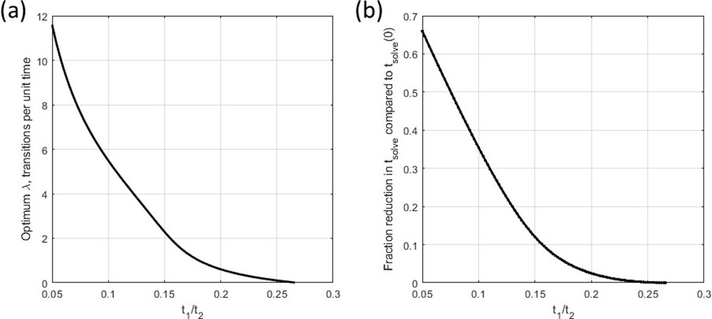
represent the respective expected “dwell times” on methods 1 and 2 if the problem is not solved. Just as in the time-limited case, we can find conditions for which a minimum average solve time exists. For values of the solve time ratio \(\frac{t_1}{t_2}\) that are less than \(\frac1{2+\sqrt{3}}\approx 0.268\), there is a positive switching tendency that minimizes the average solve time (see Figure 3). A smaller solve time ratio indicates a greater possible solve time reduction over the no-switch \((\lambda = 0)\) case and a larger optimum switching tendency \(\lambda\).

Sample Applications

In the \(n=2\) time-limited case, the threshold for switching \(\left(\frac{t_1}{t_f} < \frac12\right)\) is less strict than in the time-unlimited case \(\left(\frac{t_1}{t_2} < \frac1{2+\sqrt{3}}\right)\). There are thus more situations wherein switching is beneficial under a time limit. For instance, in a classroom exam with appropriate difficulty, the time limit and method solve times are approximately the same order of magnitude, i.e., \(t_f \sim t_i\). If a student is able to find a short method of length \(\frac{t_f}2\) or less, then a switching strategy can improve their solve probability.

On the other hand, some relevant situations do not have restrictive time limits. For example, the time limit for an undergraduate homework problem set is typically on the order of one week, but the time that is actually required to finish the set is usually on the order of three to six hours. Since \(t_f \gg t_i\), we can approximate it as a time-unlimited situation. Nevertheless, students still seek to minimize their solve time while producing a satisfactory result so they can sleep, socialize, and engage in other activities. 

The timelines of engineering design projects in industry settings also require a certain amount of strategy. Although the completion time is generally estimated at a project’s onset, it can sometimes be extended if necessary. Additionally, unforeseen circumstances—e.g., the need to pursue a new course after the original plan turned out to be nonviable, with an impractically large solve time—can necessitate a switch in techniques or methods. Given these realities, project managers aim to choose the optimal method to minimize completion time and save money.

In scenarios without a strict time limit, problem solvers should be persistent in order to optimize their outcomes, as switching methods too frequently is often quite time consuming. It only makes sense to change techniques when some methods or solution paths are very short compared to the alternatives.

Conclusions

Our model indicates that switching problem-solving methods can be beneficial even if the transitions are random, but only when at least one of the methods in question is sufficiently short. As a prerequisite, the problem solver’s toolbox must therefore contain approaches with low solve times, such as estimation or approximation techniques, a cache of existing solutions, or even an artificial intelligence assistant. 

Since a significant portion of science, technology, engineering, and mathematics coursework teaches students how to use time-consuming analysis tools, instructors should also include low solve time methods in the curriculum. Once problem solvers learn these short methods, they will be able to apply the appropriate strategies by beginning with or switching to these methods as needed. Of course, this is a general guideline, as each subject area may have its own relevant low solve time approaches. Future work can identify the way in which various techniques maximize problem-solving potential in different disciplines.

Hao Li delivered a contributed presentation on this research at the 2023 SIAM Conference on Applications of Dynamical Systems, which took place in Portland, Ore., in May 2023.

References
[1] Bahar, A., & Maker, C.J. (2015). Cognitive backgrounds of problem solving: A comparison of open-ended vs. closed mathematics problems. Eurasia J. Math. Sci. Tech. Ed., 11(6), 1531-1546.
[2] Li, H. (2023). Problem solving in engineering with multiple solution methods [Ph.D. thesis, Department of Mechanical Engineering, Massachusetts Institute of Technology]. DSpace@MIT.
[3] Linder, B.M. (1999). Understanding estimation and its relation to engineering education [Ph.D. thesis, Department of Mechanical Engineering, Massachusetts Institute of Technology]. DSpace@MIT.
[4] Shakerin, S. (2006). The art of estimation. Int. J. Eng. Educ., 22(2), 273-278.