Pythagorean Theorem on a Sphere

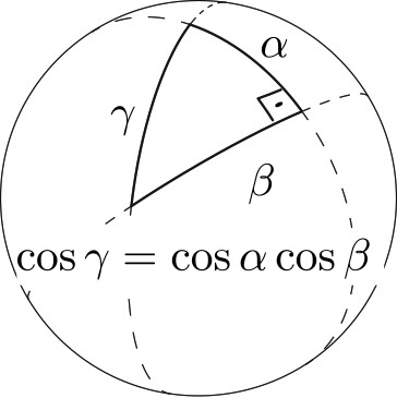
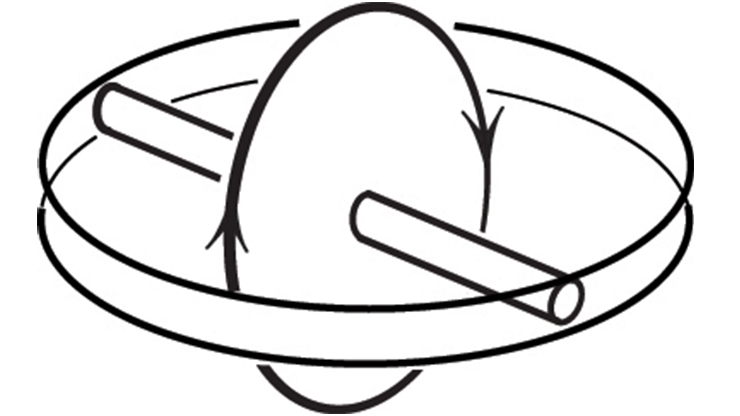
Figure 1 shows a right triangle on a unit sphere, each side being an arc of a great circle. The Pythagorean theorem on the sphere has a beautiful form:

\[\cos \alpha \cos \beta  = \cos \gamma, \tag1\]

where \(\alpha\) and \(\beta\) are the lengths of the legs and \(\gamma\) is the length of the hypotenuse.¹ Our Euclidean version is a limiting case of \((1).\)²

Several very nice and simple proofs of (1) exist, but none that I saw gave that “aha!” feeling — until I realized that the Pythagorean theorem expresses the fact that the area of a triangle is invariant under rotations around an endpoint of its hypotenuse.

To see this, let us rotate the triangle in Figure 2 around the end \(B\) of the hypotenuse with some angular velocity \(\omega.\) We can also think of rotating the whole sphere with the triangle, as one rigid object, around the radius \(OB\) (where \(O\) is the center of the sphere).

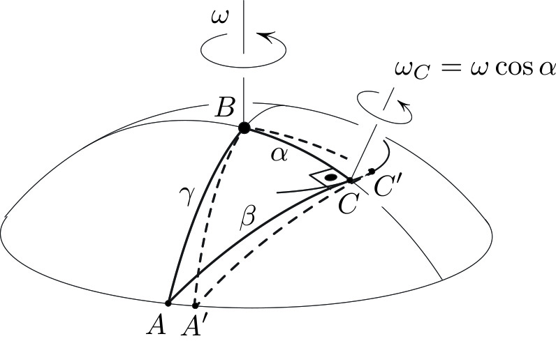
During this rotation, the area that is gained through each of the legs cancels the area that is lost through the hypotenuse, and so the rates of area gain and loss cancel each other out:

\[\boxed{\hbox{rate}_\alpha +\hbox{rate}_\beta  = \hbox{rate}_\gamma.} \tag2\]

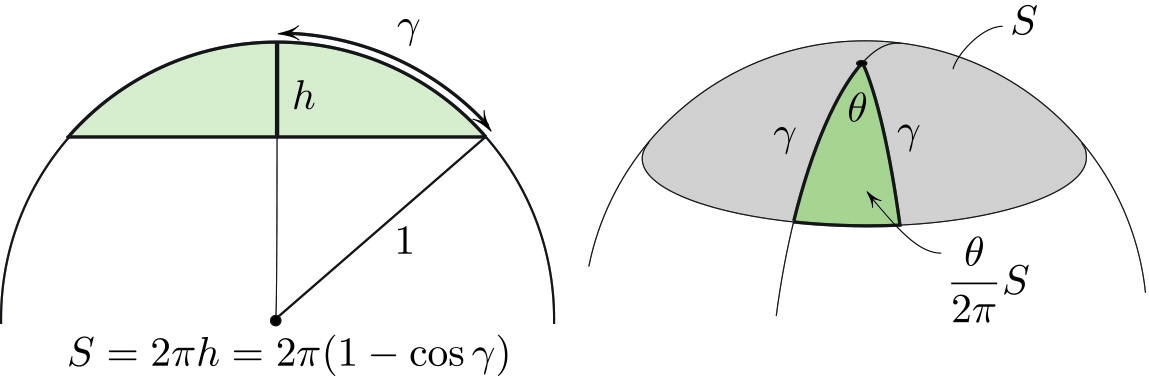
I claim that this amounts to \((1).\) Indeed, according to Figure 3, 

\[\hbox{rate}_\alpha  = \omega (1- \cos \alpha ), \ \ \hbox{rate}_\gamma = \omega ( 1- \cos \gamma). \tag3\]

Similarly, as we will see shortly,

\[\hbox{rate}_ \beta = \omega \cos \alpha (1- \cos \beta). \tag4\]

Substituting this and \((3)\) into \((2)\) and simplifying yields \((1).\)

Justification of (4)

I claim that

\[\hbox{rate}_ \beta = \omega_C(1- \cos \beta), \tag5\]

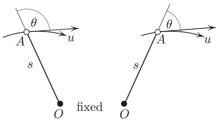
where \(\omega _C = \omega \cos \alpha\) is the angular velocity projected onto the radius \(OC.\)³ This looks just like \((3),\) but unlike in \((3),\) neither end of \(CA\) is fixed. And so to apply \((3)\) to \(AC,\) we need to say more. Thankfully, \(C\)’s velocity is tangent to \(CA\) because our triangle is right. We can therefore decompose the motion of \(CA\) into two simultaneous ones: (i) sliding along \(CA\) and (ii) pivoting on \(C.\) But since (i) does not contribute to the sweeping of area, \(\rm rate_{\beta}\) is the same as if \(C\) were fixed and \((5)\) holds by the earlier argument. And with \(\omega_C= \omega \cos \alpha\) in \((5),\) we get \((4).\)

As an aside, we can view \((2)\) as a consequence of Green’s theorem; instead of rotating the triangle, we can consider a vector field on the sphere that is given by rigid rotation around the \(OB\) axis. Then, \((2)\) expresses the vanishing of the flux through the boundary of the triangle.

We can derive the theorem of cosines on the sphere in a similar way from the area invariance.

¹ If the sphere’s radius \(R \not= 1,\) we should replace the lengths \(\alpha,\) \(\beta,\) and \(\gamma\) in \((1)\) with \(\alpha/R,\) \(\beta/R,\) and \(\gamma/R.\) Thus, \(\alpha,\) \(\beta,\) and \(\gamma\) are simply the angles between the appropriate radii of the sphere. 

² Indeed, \(\cos \alpha = 1 - \alpha ^2/2 +\ldots\) etc., and \((1)\) reduces to \(\alpha ^2 + \beta ^2 = \gamma ^2 \) to the leading order of approximation if \(\alpha\) and \(\beta\) become small. 

³ Putting it differently, as the sphere’s inhabitant at \(B\) twirls a rigid “stick” \(BC\) with angular velocity \(\omega\) (see Figure 3), the direction of the other end \(C\) rotates with \(\omega_C=\omega \cos \alpha.\) For \(C\) on the equator, \(\omega_C = 0;\) on the south pole, \(\omega_C = -\omega\) (which is not surprising, since the observer is upside down). So in a curved space, the angular velocity of a rigid object varies from point to point, unlike in the Euclidean world.

The figures in this article were provided by the author.