Randomized Linear Algebra in Scientific Computing

People often think of randomness as a nuisance — something that we must contend with, rather than fully embrace. But what if randomization could be a useful tool instead of a hinderance?

Randomized numerical linear algebra (RandNLA) is an interdisciplinary area that spans mathematics, computer science, and statistics. This exciting field uses randomization, or sketching, to reduce the computational cost of core numerical linear algebra tasks such as matrix multiplication, the solution of linear systems and least squares problems, and low-rank compression. Since matrices are ubiquitous in data science and scientific computing, advances in RandNLA can reverberate across science and engineering. During the 2025 SIAM Conference on Computational Science and Engineering (CSE25), which took place in Fort Worth, Texas, this past March, Daniel Kressner of École Polytechnique Fédérale de Lausanne delivered an invited presentation about his recent work to advance RandNLA. 

Origins and Current State of the Field

Kressner opened his CSE25 talk by tracing the origins of randomization in numerical linear algebra. It has long been common practice to use a vector with random numbers to initialize the power method and find an eigenpair. In this sense, the numerical linear algebra community has always utilized randomization, even if we did not explicitly analyze the impact of randomness. Over the last few decades, RandNLA has found new life in theoretical computer science and data science; it is now slowly starting to make its way into “mainstream” numerical analysis and scientific computing.

Kressner’s lecture highlighted randomization’s ability to accelerate computations in computational science and engineering settings. The newfound involvement of the numerical analysis community has shifted the focus away from reduced computational complexity and towards practical algorithms, numerical stability, and implementations on high-performance computing platforms. Present-day researchers are also applying RandNLA to different types of problems. For instance, data science applications require solvers for least squares and low-rank approximations, while scientific computing additionally necessitates solvers for large linear systems and the construction of surrogate models.

An impactful review article [2] introduced me to RandNLA as a Ph.D. student in 2012, and I found myself drawn to the field in subsequent years. From an algorithmic perspective, randomization is typically simple, elegant, and easy to implement; this simplicity allows users to reorganize other calculations to achieve parallelism or reutilize intermediate computations for overall computational speedup. From an analysis perspective, randomization is exciting because it involves tools from high-dimensional probability and non-asymptotic random matrix theory.

Sketching

Kressner provided a brief exposition on sketching in the context of randomization. Wikipedia defines a sketch as a “rapidly executed freehand drawing that is not usually intended as a finished work.” Similarly, a sketch of a matrix is an approximation that preserves, to an extent, the matrix’s essential features. While the term is visually evocative (I picture M.C. Escher’s Drawing Hands, a seemingly impossible sketch of two hands drawing each other), I do find it somewhat unfortunate, especially since it is the subject of several puns of algorithms that claim to be “sketchy.”

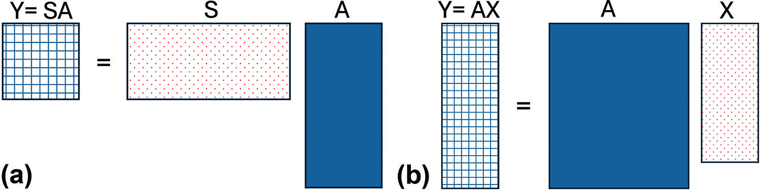
We can sketch a matrix from the left or right (see Figure 1). Suppose that we have an \(m \times n\) matrix \(A\). In low-rank approximations, sketching with an \(n \times k\) random matrix \(X\) from the right yields a sketch \(Y=AX\) that preserves the number of rows. If rank \(A\) is sufficiently low, then column space \(Y\) might be a good approximation to that of \(A\). On the other hand, least squares solvers require that the sketch preserve the number of columns, so we sketch from the left: \(Y=SA\), where \(S\) is an \(r \times m\) random matrix. The choice of random matrix \(X\) or \(S\) is quite important, and ongoing research is actively seeking random matrices that balance the cost of sketching with the accuracy of the approximation. For concreteness, we can take the random matrix to a standard Gaussian matrix — i.e., a matrix with independent and identically distributed normal random variables that have zero mean and unit variance. This action typically yields the strongest theoretical guarantees. Several excellent surveys on sketching are available in the literature [2-5, 7].

Randomization for the Solution of Linear Systems

Kressner shared many success stories of randomization in surrogate model construction, linear system solutions, time integration, families of matrices, and subset selection. While each topic is fascinating in its own right, I will focus on his work with linear systems. This subject also prompted the largest number of audience questions at CSE25.

In scientific computing, we must often solve large linear systems \(Au=b\), where the size of matrices \(A\) can be in the millions or billions. These problems arise in the context of numerical solutions to partial differential equations (PDEs). Kressner explored the solution of sequences of linear systems \(A_iu_i=b_i\) for \(i=1,...,n\), where the coefficient matrices \(A_i\) have dimension \(d \times d\) and change only slightly from system to system. Such linear systems might arise from the discretization of time-dependent PDEs with variable time stepping. The development of direct and iterative solvers for large linear systems remains an important area of research. Several existing iterative solvers—such as the conjugate gradient method or the generalized minimal residual method (GMRES)—can generate sequences of iterates to approximate a linear system’s solution.

When solving sequences of linear systems, we must consider the reuse of information from one linear system solution to another. Potential approaches include constructing an intelligent initial guess (sometimes called warm starting), extracting a solution basis from the previous iteration (i.e., recycling and augmented methods), or reusing/updating a preconditioner [6].

Kressner presented an approach [1] that somewhat used randomization to generate a good initial guess. The main idea is quite simple. Suppose that we solved \(m-1\) linear systems and collected the solutions into a so-called snapshot matrix \(U=[u_1 \enspace ... \enspace u_{m-1}]\). In many cases, the snapshot matrix has rapidly decaying singular values and can be well approximated by a low-rank matrix — a key idea in reduced order modeling, e.g., proper orthogonal decomposition (POD). We can sketch the solution to the first \(m\) system as \(Y=UX\), where \(X\) is a random matrix. To generate a new initial guess, we must then consider an approximation of the form \(Y \, z\), where \(z\) is a solution to the linear least squares problem

\[\underset{z}{\min}\|A_mY\,z-b_m\|_2\]

for the optimal solution \(z^*_m\). Next, we can seed an iterative method like GMRES with the initial guess \(Y\,z^*_m\). Computing \(A_mY\) and solving the least squares problem requires computational effort, though Kressner argued that doing so is often much cheaper than existing methods to accelerate linear solvers. He also maintained that orthogonalizing \(Y\)—as in POD or randomized singular value decomposition—is unnecessary.

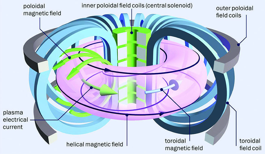
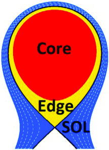
To demonstrate, Kressner presented numerical results from an application in plasma physics. He considered the simulation of plasma turbulence in the outermost plasma region of a tokamak fusion reactor, where the plasma comes in contact with the surrounding external solid walls (see Figures 2 and 3). This application, which has multiscale physics in space and time, requires the solution of a sequence of linear systems that arise from discretized fluid equations coupled with Maxwell’s equations for electromagnetics. The aforementioned method [1] led to a \(3\times\) speedup in wall-clock time as compared to the baseline approach (see Figure 4). In other applications that involve elliptic PDEs, this technique can produce \(10\times\) speedups in wall-clock time.

Kressner also discussed iterative methods for large linear systems that arise from kernel matrices in system identification. The linear system is \((I+K)u=b\), where \(K\) is a kernel matrix and \(I\) is the identity matrix. Kressner suggested augmenting \(b\) with a few (fictitious) random vectors as \(B=[b,x]\), where \(X\) contains random vectors, and solving the block system \((I+K)U=B\). He contends that this approach is more beneficial—despite increasing the computational cost per iteration—because the addition to the right side implicitly preconditions the system, which intuitively leads to improved convergence.

The talk itself was well received by the CSE25 audience. If we measure a presentation’s popularity by the number of photos that attendees take of slides, Kressner’s fast-paced delivery meant that phone and tablet cameras were active throughout the session. Kressner—mindful of the Friday morning audience—kept the analysis to a minimum, included compelling graphics, and provided profound insight into randomization. He addressed a truly impressive number of RandNLA applications that spoke to his oeuvre.

Outlook

Kressner concluded with randomization’s outlook in scientific computing, noting the myriad opportunities for researchers in RandNLA. From a theoretical perspective, randomization can benefit from new ideas in high-dimensional probability and random matrix theory. As the field matures, it will need robust software that can handle the current demands of data science and scientific computing. The impact of numerical linear algebra libraries—such as LAPACK—on science and engineering cannot be overstated, and the development of a similar library for RandNLA is ongoing [5]. Another important direction involves the adaptation of existing algorithms to new applications and the creation of novel algorithms based on the challenges and needs of modern use cases. While it may be impossible (or in my case, undesirable) to completely eliminate randomness from our lives, in scientific computing we can at least embrace it gracefully.

Acknowledgments: The author would like to thank Ilse Ipsen and Daniel Kressner for their feedback on this article.

References
[1] Guido, M., Kressner, D., & Ricci, P. (2024). Subspace acceleration for a sequence of linear systems and application to plasma simulation. J. Sci. Comput., 99(3), 68.
[2] Halko, N., Martinsson, P.-G., & Tropp, J.A. (2011). Finding structure with randomness: Probabilistic algorithms for constructing approximate matrix decompositions. SIAM Rev., 53(2), 217-288.
[3] Mahoney, M.W. (2011). Randomized algorithms for matrices and data. Found. Trends Mach. Learn., 3(2), 123-224.
[4] Martinsson, P.-G., & Tropp, J.A. (2020). Randomized numerical linear algebra: Foundations and algorithms. Acta Numer., 29, 403-572.
[5] Murray, R., Demmel, J., Mahoney, M.W., Erichson, N.B., Melnichenko, M., Malik, O.A., … Dongarra, J. (2023). Randomized numerical linear algebra: A perspective on the field with an eye to software (Technical report no. UCB/EECS-2023-19). Berkeley, CA: University of California, Berkeley.
[6] Soodhalter, K.M., de Sturler, E., & Kilmer, M.E. (2020). A survey of subspace recycling iterative methods. GAMM-Mitteilungen, 43(4), e202000016.
[7] Woodruff, D.P. (2014). Sketching as a tool for numerical linear algebra. Found. Trends Theor. Comput. Sci., 10(1-2), 1-157.