Removing Kalman from Ensemble Kalman Filtering
Jeff Anderson builds forecast systems for the U.S. National Center for Atmospheric Research in Boulder, Co. He began his invited talk at the 2021 SIAM Conference on Computational Science and Engineering, which took place virtually earlier this year, with a potentially unsettling threat: he would remove the “Kalman” from ensemble Kalman filtering.
Anderson’s objective was hardly a personal vendetta. A forecast system assimilates weather forecasts from models and weather observations from instruments, uses the observations to reduce inevitable errors in the predicted state, and feeds this improved state vector to the prediction model as the initial condition for its next run. In precise mathematical terms, the Kalman filter is the best tool for predicting a system’s state (and the probability density function of that state) from noisy observations of its past, given linear process models and additive Gaussian noise in processes and measurements, among other conditions.

When all of these particular conditions are fulfilled, Kalman can compare the system model’s prediction of what should happen with the system’s observations of what did happen — fully exploiting the requirement that should and did are subject to Gaussian error. This comparison can filter the noise that disrupts a model’s predictions and the errors that corrupt the associated measurements to produce the most accurate estimate of a system’s present state and its corresponding covariance matrix.
If Kalman is mathematically the best possible filter for the heart of a weather forecasting system, why should Anderson want it removed? Simply put, the hundreds of millions of state variables in large Earth system models induce computational congestive heart failure. The mathematical derivation of the classic Kalman filter is a relatively straightforward exercise that involves inverses of covariance matrices. Computationally, inverting matrices means solving linear systems — a task whose workload grows faster than the square of the number of variables.
Rather than excising Kalman by radical surgery, Anderson characterized his approach as “an evolutionary attempt to eliminate the assumptions” that were made when the Kalman filter was developed. The evolutionary steps that he outlined amount to the one-by-one removal of some formerly essential requirements: a linear model to advance the covariance estimate, a linear forward operator, an unbiased estimate of covariance, an unbiased model prior, and (almost) a Gaussian prior.
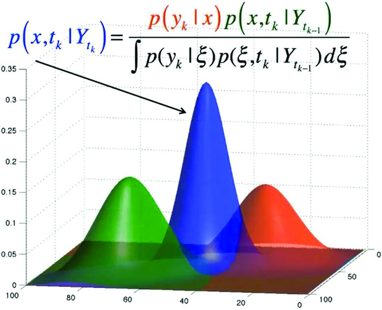
Setting the stage for his reductive strategy, Anderson offered a graphic depiction of the filtering challenge (see Figure 1). The two-dimensional state variable is in the horizontal plane. The prior distribution in green signifies the outcome of the previous predictive step, and the likelihood in red captures what the instrument makers know about the uncertainty in their observations.
Mathematically speaking, the posterior in blue is the product of the prior with the likelihood, which is normalized by the denominator of the expression in Figure 1. Computationally, one calculates the statistics of the posterior state estimate—the shape of the blue surface—by solving large linear systems that are built from covariance matrices. On a geophysical scale, the dual burdens of storage and computational cost are prohibitive.

To avoid the expense of solving Kalman’s enormous linear systems, Anderson introduced an ensemble of smaller elements that ultimately capture the original system’s critical features. Imagine the prior state distribution (the green component in Figure 1) as a surface that was fit to an ensemble of prior states — a set of well-selected points in the horizontal plane. Next, advance each member of this prior ensemble a single time step to a posterior with the same mean and covariance as the blue posterior surface in Figure 1.
From a practical standpoint, Anderson and his colleagues have shown that constructing and advancing such an ensemble is entirely feasible. A deterministic update of a single observed variable “can compute the impact of an observation on each state variable independently,” he said. Anderson used the measurement error likelihood to shift the observed variable, then calculated the corresponding shift in the weakly correlated unobserved state variable. The process amounts to regressing shifts in the observed variable onto shifts in the unobserved variable.
This process repeats when all ensemble members have been updated. Because the regression of observation increments onto state variable increments can be performed independently, computations can be distributed across the nodes of a parallel machine to attain even faster analyses.
Anderson approaches ensemble filtering with the realization that “making the core problem simpler allows you to introduce added complexity” at a later time, he said. Certainly, this ensemble formulation avoids both massive matrix inversions and the requirement of linear relations between observations and states.
Anderson presented two computational data assimilation experiments that are examples of such “added complexity.” Both utilize the Lorenz 96 40-variable system: \(dX_i/dt=(X_i+1-X_i-2)X_i-1-X_1+F\). It behaves a bit like models of the weather within bands of latitude around the Earth. One experiment explored data localization (biased covariance) and the other dealt with model errors (biased model prior).

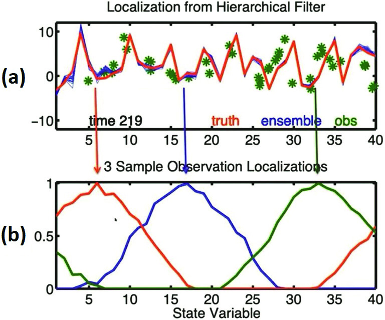
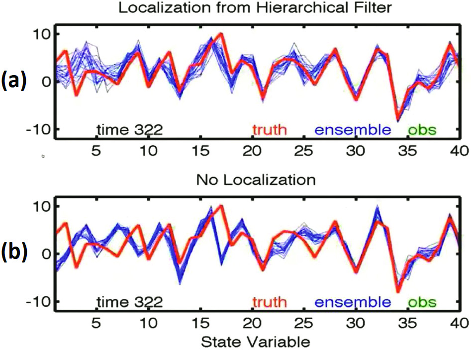
Data like temperature observations in Denver, Co., is obviously more important to temperature prediction in Boulder than an observation from Antarctica. Anderson used simulations with the Lorenz 96 40-variable system to illustrate the success of localizing observations. Figure 2a depicts an early stage of a set of these simulations; the red curve is the “truth” and each green asterisk is an observed value that is collected at its location along the horizontal axis. Figure 2b displays the local weighting of three of these observations, and Figure 3 demonstrates the power of such a localization after a few hundred more iterations. The blue localized ensemble predictions in Figure 3a hew closely to the red “truth,” while the blue unweighted predictions in 3b deviate wildly.
Computational weather models are inherently inaccurate because of finite-precision arithmetic, if nothing else. Anderson and his colleagues mimicked model error by changing the forcing constant \(F\) in the Lorentz 96 system. Subsequent simulations demonstrated the success of an adaptive approach for managing model bias.
Other work has explored non-Gaussian priors, which might arise from observations of a trace chemical’s concentration and can never be negative. Methods to reduce some of the additional restrictions and limitations of ensemble filtering—such as the need for regression to increment state variables—are currently under study.
Despite the progress that he reported, Anderson made clear that enabling ensemble filtering on a geophysical scale is far from done and dusted. Future directions might include particle filters, their formidable computational costs notwithstanding. “Lots of fun is still left in merging ensemble and particle filters,” Anderson said.
About the Author
Paul Davis
Professor emeritus, Worcester Polytechnic Institute
Paul Davis is a professor emeritus of mathematical sciences at Worcester Polytechnic Institute.
Stay Up-to-Date with Email Alerts
Sign up for our monthly newsletter and emails about other topics of your choosing.


