Resilient Data-driven Dynamical Systems with Koopman: An Infinite-dimensional Numerical Analysis Perspective

Dynamical systems, which describe the evolution of systems in time, are ubiquitous in modern science and engineering. They find use in a wide variety of applications, from mechanics and circuits to climatology, neuroscience, and epidemiology. Consider a discrete-time dynamical system with state \(\boldsymbol{x}\) in a state space \(\Omega\subset\mathbb{R}^d\) that is governed by an unknown and typically nonlinear function \(\boldsymbol{F}:\Omega\rightarrow\Omega\):

\[\boldsymbol{x}_{n+1} = \boldsymbol{F}(\boldsymbol{x}_n), \qquad n\geq 0. \tag1\]

The classical, geometric way to analyze such systems—which dates back to the seminal work of Henri Poincaré—is based on the local analysis of fixed points, periodic orbits, stable or unstable manifolds, and so forth. Although Poincaré’s framework has revolutionized our understanding of dynamical systems, this approach has at least two challenges in many modern applications: (i) Obtaining a global understanding of the nonlinear dynamics and (ii) handling systems that are either too complex to analyze or offer incomplete information about the evolution (i.e., unknown, high-dimensional, and highly nonlinear \(\boldsymbol{F}\)).

Koopman operator theory, which originated with Bernard Koopman and John von Neumann [6, 7], provides a powerful alternative to the classical geometric view of dynamical systems because it addresses nonlinearity: the fundamental issue that underlies the aforementioned challenges. We lift the nonlinear system \((1)\) into an infinite-dimensional space of observable functions \(g:\Omega\rightarrow\mathbb{C}\) via a Koopman operator \(\mathcal{K}\):

\[\mathcal{K}g(\boldsymbol{x}_n) = g(\boldsymbol{x}_{n+1}).\]

The evolution dynamics thus become linear, allowing us to utilize generic solution techniques that are based on spectral decompositions. In recent decades, Koopman operators have captivated researchers because of emerging data-driven and numerical implementations that coincide with the rise of machine learning and high-performance computing [2].

One major goal of modern Koopman operator theory is to find a coordinate transformation with which a linear system may approximate even strongly nonlinear dynamics; this coordinate system relates to the spectrum of the Koopman operator. In 2005, Igor Mezić introduced the Koopman mode decomposition [8], which provided a theoretical basis for connecting the dynamic mode decomposition (DMD) with the Koopman operator [9, 10]. DMD quickly became the workhorse algorithm for computational approximations of the Koopman operator due to its simple and highly extensible formulation in terms of linear algebra, and the fact that it applies equally well to data-driven modeling when no governing equations are available. However, researchers soon realized that simply building linear models in terms of the primitive measured variables cannot sufficiently capture nonlinear dynamics beyond periodic and quasi-periodic phenomena. A major breakthrough occurred with the introduction of extended DMD (EDMD), which generalizes DMD to a broader class of basis functions in which to expand eigenfunctions of the Koopman operator [11]. One may think of EDMD as a Galerkin method to approximate the Koopman operator by a finite matrix \(\mathbf{K}\in\mathbb{C}^{N\times N}\).

However, practical realities have tempered much of the promise of Koopman theory — infinite-dimensional spectral problems are difficult! So difficult, in fact, that sometimes a computer cannot even approximately solve them. Two of the biggest challenges that currently face data-driven Koopman theory are as follows [2]:

(i) Spectral pollution (i.e., spurious modes) that results from the approximation of infinite-dimensional dynamics in a chosen finite-dimensional computational basis
(ii) Systems with continuous eigenvalue spectrums, such as a simple pendulum that oscillates at a continuous range of frequencies for different energies. 

Moreover, if \(\mathcal{K}\) preserves a key structure (e.g., a measure), can we ensure that \(\mathbf{K}\) does so as well? Here, we summarize these significant challenges and describe new advances that offer resilient solutions that are based on rigorous, infinite-dimensional numerical analysis [3-5].

Addressing Spectral Pollution: The Power of Residuals

We want to approximate functions \(g\) in terms of a finite set of basis functions \(\psi_1,\ldots,\psi_N\), \(\psi_j:\Omega\rightarrow\mathbb{C}\). In turn, EDMD approximates \(\mathcal{K}\) by a finite matrix \(\mathbf{K}\in\mathbb{C}^{N\times N}\). Due to this truncation, eigenvalues of \(\mathbf{K}\) may be spurious and have no relationship to the spectrum of \(\mathcal{K}\). Consider trajectory data \(\{\color{blue}{\boldsymbol{x}^{(m)}}, \color{green}{\boldsymbol{y}^{(m)}}=\boldsymbol{F}(\color{blue}{\boldsymbol{x}^{(m)}})\}^M_{m=1}\) and define the matrices

\[\color{blue}{ M_X=\sqrt{W} \begin{pmatrix} \psi_1(\boldsymbol{x}^{(1)})& \cdots & \psi_N(\boldsymbol{x}^{(1)})\\ &\vdots&\\ \psi_1(\boldsymbol{x}^{(M)})& \cdots & \psi_N(\boldsymbol{x}^{(M)}) \end{pmatrix}},\] \[\color{green}{M_Y= \sqrt{W} \begin{pmatrix} \psi_1(\boldsymbol{y}^{(1)})& \cdots & \psi_N(\boldsymbol{y}^{(1)})\\ &\vdots&\\ \psi_1(\boldsymbol{y}^{(M)})& \cdots & \psi_N(\boldsymbol{y}^{(M)}) \end{pmatrix}},\] 

where \(W=\textrm{diag}(w_1,\ldots w_M)\). The parameters \(w_M\), which we interpret as quadrature weights, measure the relative importance of each snapshot \((\color{blue}{\boldsymbol{x}^{(m)}}, \color{green}{\boldsymbol{y}^{(m)}})\) and \(\mathbf{K}=(\color{blue}{M_X}{}^*\color{blue}{M_X})^\dagger \color{blue}{M_X}{}^*\color{green}{M_Y}\). How can we assess the accuracy of a candidate eigenfunction \(\varphi(x)=\Sigma_{j=1}^N\boldsymbol{v}_j\psi_j(x)\) of \(\mathcal{K}\) with \(\boldsymbol{v}\in\mathbb{C}^N\) and a corresponding candidate eigenvalue \(\lambda\)? (Note that we may compute such approximate eigenpairs from \(\mathbf{K}\) or some other means). One solution is to approximate relative residuals via the equation 

\[\frac{\|\mathcal{K}\varphi-\lambda \varphi\|^2}{\|\varphi\|^2}\approx \frac{\boldsymbol{v}^*[\color{green}{M_Y}{}^*\color{green}{M_Y}-\lambda(\color{blue}{M_X}{}^*\color{green}{M_Y})^* - \overline{\lambda}\color{blue}{M_X}{}^*\color{green}{M_Y}+|\lambda|^2\color{blue}{M_X}{}^*\color{blue}{M_X}]\boldsymbol{v}}{\boldsymbol{v}^*[\color{blue}{M_X}{}^*\color{blue}{M_X}]\boldsymbol{v}}.\] 

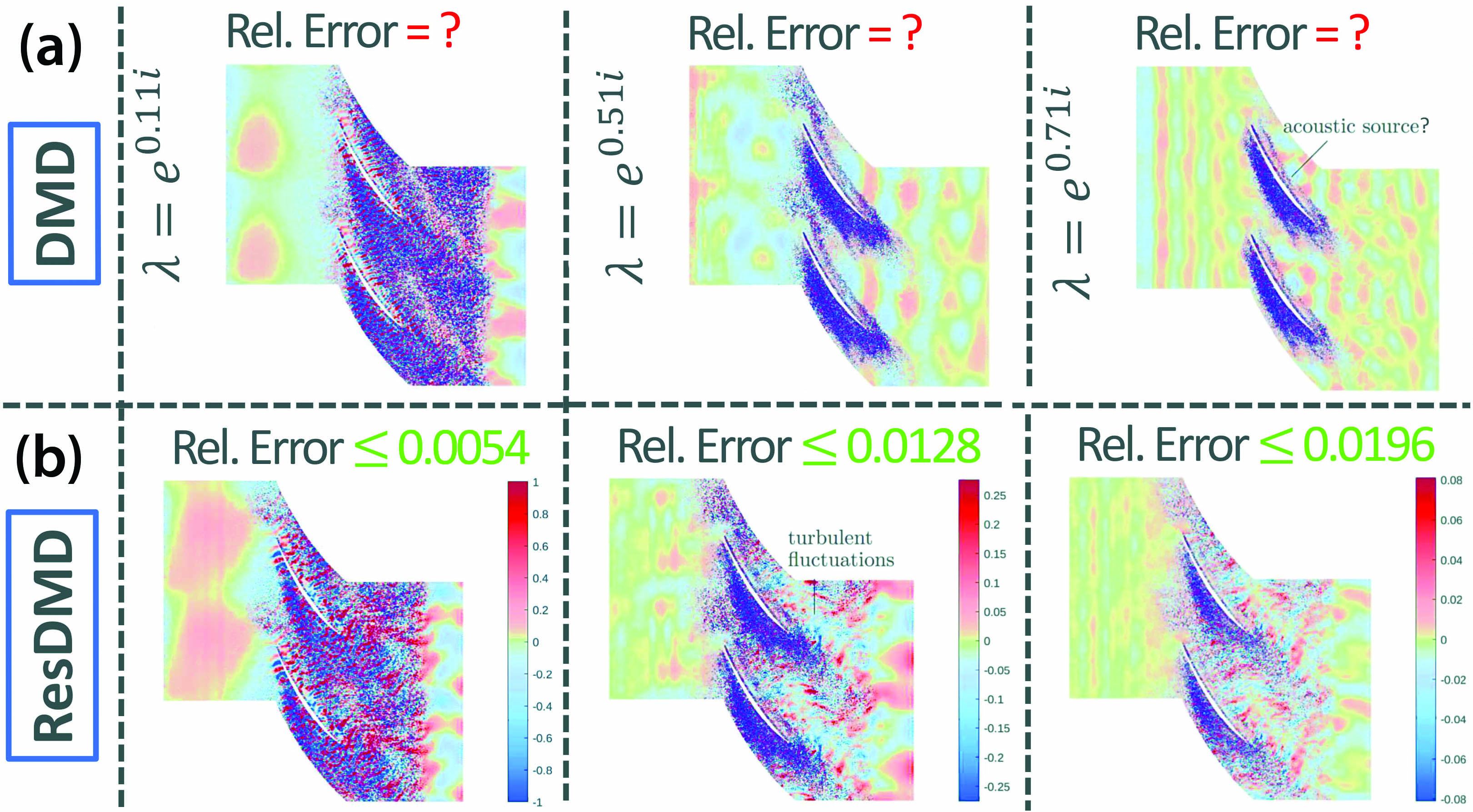
Under generic conditions, this approximation becomes exact in the large data limit \(M\rightarrow\infty\). Using the additional matrix \(\color{green}{M_Y}{}^*\color{green}{M_Y}\) provides access to an infinite-dimensional residual, even with finite matrices. We can therefore turn this idea into an algorithm—residual DMD (ResDMD) [5]—at no extra computational or data cost beyond that of EDMD. By either discarding eigenpairs of \(\mathbf{K}\) with large residuals or using the residual itself to search for local minima, we can compute spectra of \(\mathcal{K}\) without spectral pollution. For example, Figure 1 illustrates Koopman modes that are computed for a turbulent flow; ResDMD provides error bounds and hence allows us to compute a picture that is physically correct. Because ResDMD verifies spectral computations, we can also verify Koopman mode decompositions and learned choices of \(\psi_j\).

Computing Continuous Spectra: Smoothing with Rational Kernels

Many operators in infinite dimensions can have continuous spectra and thus may not be diagonalized by eigenfunctions alone. However, truncating to a finite matrix \(\mathbf{K}\) destroys continuous spectra. We wish to compute so-called spectral measures, as doing so allows us to provide a diagonalization of \(\mathcal{K}\). If the dynamical system preserves a measure, we can expand a function \(g:\Omega\rightarrow\mathbb{C}\) in terms of eigenfunctions \(\varphi_j\) and generalized eigenfunctions \(\phi_{\theta,g}\) of \(\mathcal{K}\) [8]:

\[g(\boldsymbol{x})=\sum_{\text{eigs.} \; \lambda_j}c_j \varphi_j(\boldsymbol{x})+\underbrace{\int_{\pi}^\pi \phi_{\theta,g}(\boldsymbol{x}) d\theta}_{\text{continuous spectra}}.\]

This decomposition is characterized by spectral measures \(\nu_g\) that are supported on the unit circle. Just as a prism splits white light into its different frequencies (see Figure 2a), \(\nu_g\) splits the signal \(\{g(\boldsymbol{x}_n)\}\) into simpler parts with corresponding spectral frequencies:

\[g(\boldsymbol{x}_n)=[\mathcal{K}^ng](\boldsymbol{x}_0)=\sum_{\text{eigs.} \: \lambda_j}c_j \lambda_j^n\varphi_j(\boldsymbol{x}_0)+\int_{\pi}^\pi e^{in\theta}\phi_{\theta,g}(\boldsymbol{x}_0) d\theta.\] 

We can compute smoothed approximations \(\nu_g^{\epsilon}\) that correspond to the convolution of \(\nu_g\) with a smoothing kernel of smoothing parameter \(\epsilon\) [5]. A judicious choice of rational kernels leads to an exact representation of \(\nu_g^{\epsilon}\) in terms of the resolvent operator, i.e., solutions of linear systems \((\mathcal{K}-z)^{-1}g\). We must adaptively select the truncation size \(N=N(\epsilon)\) to compute the solutions of these systems for a given smoothing parameter \(\epsilon\). This action yields an algorithm that computes spectral measures of generic Koopman operators [5] with explicit convergence rates as \(\epsilon\downarrow 0\), which allows us to compute continuous spectra of Koopman operators. Figure 2 depicts this algorithm in action for the nonlinear pendulum, which is readily analyzable via Poincaré’s geometric approach but remained a canonical open problem in Koopman analysis for several years.

Structure-preserving Discretizations

We can also enforce structure preservation in approximations of Koopman operators. For example, if the system in \((1)\) is measure preserving, then \(\mathcal{K}\) is an isometry. When \(G=\color{blue}{M_X}{}^*\color{blue}{M_X}\), \(\boldsymbol{g}^*\mathbf{K}^*G\mathbf{K}\boldsymbol{g}\approx\|\mathcal{K}g\|^2=\|g\|^2\approx \boldsymbol{g}^*G\boldsymbol{g}\), which becomes exact in the large data limit. Measure-preserving EDMD (mpEDMD) [3] enforces \(G=\mathbf{K}^*G\mathbf{K}\) and leads to an orthogonal Procrustes problem:

\[\mathbf{K}\in\underset{\underset{B^*GB=G}{B\in\mathbb{C}^{N\times N}}}{\textrm{argmin}}\left\|\color{green}{M_Y} G^{-\frac{1}{2}}-\color{blue}{M_X} BG^{-\frac{1}{2}}\right\|_F^2. \tag2\]

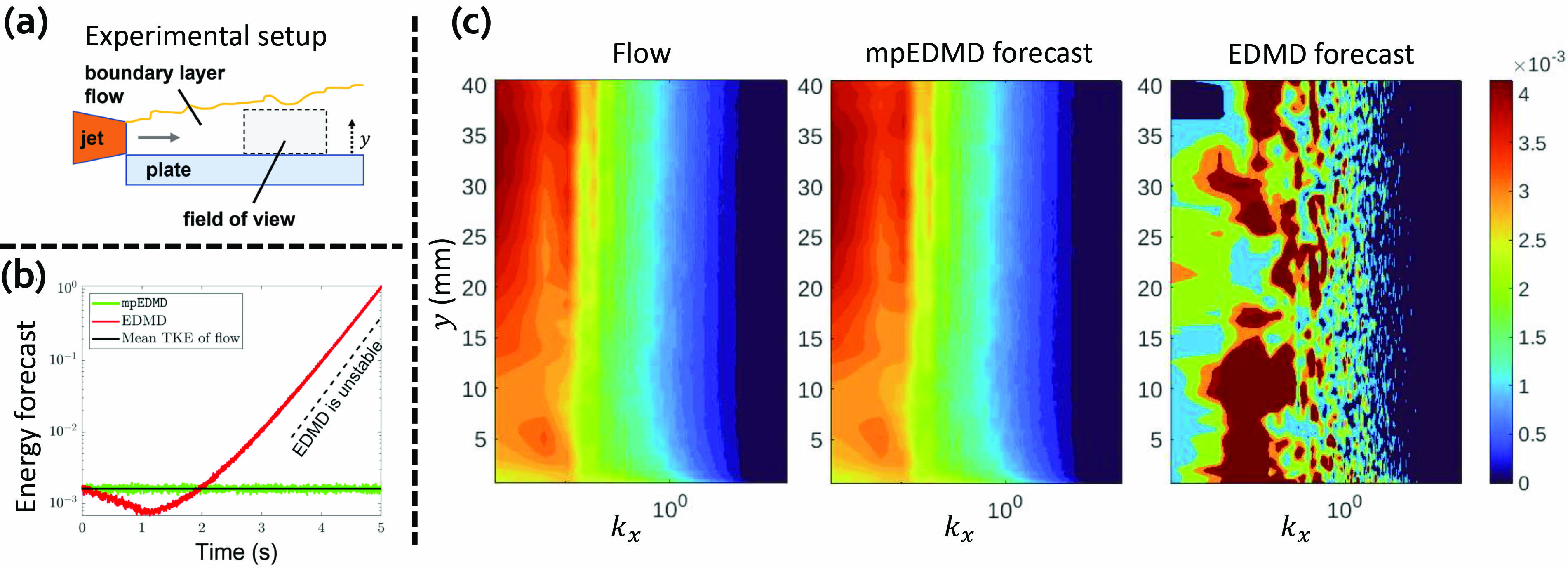
Using the singular value decomposition, we can compute a solution; this solution combines a Galerkin projection with a polar decomposition. For information about incorporating other types of constraints in DMD via Procrustes problems, see [1]. Figure 3 shows key benefits of mpEDMD when capturing the behavior of a turbulent boundary-layer flow. Moreover, mpEDMD utilizes a discretization matrix that is normal in a suitable Hilbert space, thus allowing us to tackle the two aforementioned challenges and causing the convergence of key spectral properties and even convergence rates in system sizes \(N\). The problem in \((2)\) is also equivalent to the corresponding constrained total least-squares problem and hence provides a strongly consistent estimation that is robust to noise in \(\color{blue}{M_X}\) and \(\color{green}{M_Y}\).

The Need for Infinite-dimensional Numerical Analysis

These examples demonstrate the way in which an infinite-dimensional numerical analysis view of spectral computations led to breakthroughs in the use of Koopman operators. But this is by no means the end of the story, as future directions involve establishing connections to infinite-dimensional control theory and optimizing feature spaces based on measures of a subspace’s invariance. However, any theory that seeks to understand the convergence of algorithms for Koopman operators—and any algorithm that is based on finite-dimensional approximations and seeks to be robust—must be aware of the infinite-dimensional nature of Koopman operators and the associated pitfalls.

Given the rich history of spectral computations, it is natural to turn to infinite-dimensional numerical analysis for methods and solutions. However, we cannot solve all infinite-dimensional spectral problems computationally, and the same is undoubtedly true for data-driven dynamical systems. The establishment of methodological boundaries—i.e., proving impossibility results that shine a light on limitations and guide us in feasible directions—will be a key future direction in this field. A formidable question is, “What are the foundations of data-driven dynamical systems and computing spectral properties of Koopman operators?” The answer will help us realize Koopman’s 90-year-old perspective as a powerful tool in the 21st century.

References

[1] Baddoo, P.J., Herrmann, B., McKeon, B.J., Kutz, J.N., & Brunton, S.L. (2021). Physics-informed dynamic mode decomposition (piDMD). To appear in Proc. Royal Soc. A.
[2] Brunton, S.L., Budišić, M., Kaiser, E., & Kutz, J.N. (2022). Modern Koopman theory for dynamical systems. SIAM Rev., 64(2), 229-340.
[3] Colbrook, M.J. (2022). The mpEDMD algorithm for data-driven computations of measure-preserving dynamical systems. Preprint, arXiv:2209.02244.
[4] Colbrook, M.J., Ayton, L.J., & Szőke, M. (2022). Residual dynamic mode decomposition: Robust and verified Koopmanism. Preprint, arXiv:2205.09779.
[5] Colbrook, M.J., & Townsend, A. (2021). Rigorous data-driven computation of spectral properties of Koopman operators for dynamical systems. Preprint, arXiv:2111.14889.
[6] Koopman, B.O. (1931). Hamiltonian systems and transformation in Hilbert space. Proc. Nat. Acad. Sci., 17(5), 315-318.
[7] Koopman, B.O., & Von Neumann, J. (1932). Dynamical systems of continuous spectra. Proc. Nat. Acad. Sci., 18(3), 255-263.
[8] Mezić, I. (2005). Spectral properties of dynamical systems, model reduction and decompositions. Nonlin. Dyn., 41(1), 309-325.
[9] Rowley, C.W., Mezić, I., Bagheri, S., Schlatter, P., & Henningson, D.S. (2009). Spectral analysis of nonlinear flows. J. Fluid Mech., 641, 115-127.
[10] Schmid, P.J. (2010). Dynamic mode decomposition of numerical and experimental data. J. Fluid Mech., 656, 5-28.
[11] Williams, M.O., Kevrekidis, I.G., & Rowley, C.W. (2015). A data-driven approximation of the Koopman operator: Extending dynamic mode decomposition. J. Nonlin. Sci., 25(6), 1307-1346.