Scientific Machine Learning: How Julia Employs Differentiable Programming to Do it Best

Julia, an advanced dynamic programming language for numerical computing, has solved the “two-language problem” by allowing developers to write low-level, high-performance code and high-level “scripting” code in a single language. It is significantly faster than Python and R, and considerably more productive than C, C++, and Fortran. In addition to these successes, Julia continues to bring novel technologies to computational scientists. One of its most exciting new capabilities is differentiable programming (\(\partial \textrm{P}\)). Recent work to leverage Julia’s compiler allows for the computation of efficient and accurate derivatives of arbitrary Julia programs. This is no mere party trick; program differentiation enables scientists to combine modern machine learning with the computational models developed from centuries of domain knowledge. Much as Julia provides the best of productivity and performance, \(\partial \textrm{P}\) offers scientific programmers tremendous benefits—in terms of both performance and accuracy—over black box approaches to machine learning.

At first glance, a casual practitioner might think that scientific computing and machine learning are different fields. Modern machine learning has made its mark through breakthroughs in neural networks. The applicability of such networks to solving a large class of difficult problems has led to the design of new hardware and software that process extremely high quantities of labeled training data while simultaneously deploying trained models in devices. In contrast, scientific computing—a discipline as old as computing itself—tends to use a broader set of modeling techniques that arise from underlying physical phenomena. Compared to the typical machine learning researcher, computational scientists generally work with smaller volumes of data but more computational range and complexity. However, deeper similarities emerge if we move beyond this superficial analysis. Both scientific computing and machine learning would be better served by the ability to differentiate, rather than the building of domain-specific frameworks. This is the purpose of \(\partial \textrm{P}\).¹

\(\partial \textrm{P}\) concerns computing derivatives in the sense of calculus. Scientists have calculated derivatives since Isaac Newton’s time, if not before, and machine learning has now made them ubiquitous in computer science. Derivatives power self-driving cars, language translation, and many engineering applications. Most researchers have likely written derivatives—often painfully by hand—in the past, but derivatives for scientific challenges are increasingly beyond reach.

Julia’s approach has one overarching goal: enable the use domain-specific scientific models as an integral part of researchers’ machine learning stack. This can be in place of—or in addition to—big training sets. The idea is profoundly compelling, as these models embody centuries of human intelligence. Julia makes it possible for scientists to apply state-of-the-art machine learning without discarding hard-won physical knowledge. In a recent blog post, Chris Rackauckas discusses the essential tools of modern scientific machine learning and finds Julia to be the language best suited for scientific machine learning [2].

Julia can perform automatic differentiation (AD) on eigensolvers, differential equations, and physical simulations. Loops and branches do not present obstacles. Researchers calculate derivatives in customized ways for a variety of problem areas, yet \(\partial \textrm{P}\) can greatly simplify the experience. We list a few and invite readers to share more:

1. Surrogate modeling: Running scientific simulations is often expensive because they evaluate systems using first principles. Allowing machine learning models to approximate the input-output relation can accelerate these simulations. After training neural networks or other surrogate models on expensive simulations once, researchers can use them repeatedly in place of the simulations themselves. This lets users explore the parameter space, propagate uncertainties, and fit the data in ways that were previously impossible.

2. Adjoint sensitivity analysis: Calculating the adjoint of an ordinary differential equation (ODE) system requires solving the reverse ODE \(\lambda'=\lambda'\)*df/du+df/dp. The term \(\lambda'\)*df/du is the primitive of backpropagation. Therefore, applying machine learning AD tooling to the ODE function \(f\) accelerates the scientific computing adjoint calculations.

3. Inverse problems: For many parameterized scientific simulations, researchers speculate about the parameters that would make their model best fit. This pervasive inverse problem is difficult because it requires the gradient of a large, existing simulation. One can train a model on a simulator, then use the simulator to quickly solve inverse problems. However, doing so requires generating massive amounts of data for training, which is computationally expensive. Scientists can learn much more quickly and efficiently by differentiating via simulators.

4. Probabilistic programming: Inference on statistical models is a crucial tool. Probabilistic programming enables more complex models and scaling to huge data sets by combining statistical methods with the generality of programming constructs. While AD is the backbone of many probabilistic programming tools, domain-specific languages lack access to an existing ecosystem of tools and packages. In a general-purpose language, \(\partial \textrm{P}\) has the benefit of higher composability, access to better abstractions, and richer models.

Julia’s flexible compiler—which can turn generic, high-level mathematical expressions into efficient native machine code—is ideal for \(\partial \textrm{P}\). The Zygote.jl and Cassette.jl packages provide a multipurpose system for implementing reverse-mode AD, whereas ForwardDiff.jl provides forward mode. Julia runs efficiently on central processing units, graphics processing units (GPUs), parallel computers, and Google TPUs (tensor processing units), and is ready for future processors. Because of its composability, the combination of two packages that respectively offer the ability to conduct \(\partial \textrm{P}\) and run on GPUs automatically yields the capacity to perform \(\partial \textrm{P}\) on GPUs without additional effort.

\(\partial \textrm{P}\): Differentiate Programs, not Formulas: \(\sin(x)\) Example

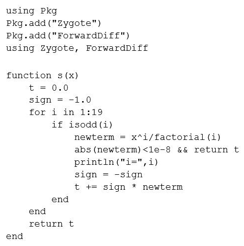
We begin with a very simple example to differentiate \(\sin(x)\), written as a program through its Taylor series:

\[\sin(x)=x-\frac{x^3}{3!} + \frac {x^5}{5!}- \dotsb \]

The number of terms is not fixed, but instead depends on \(x\) through a numerical convergence criterion. This runs on Julia v1.1 or higher (see Figure 1).

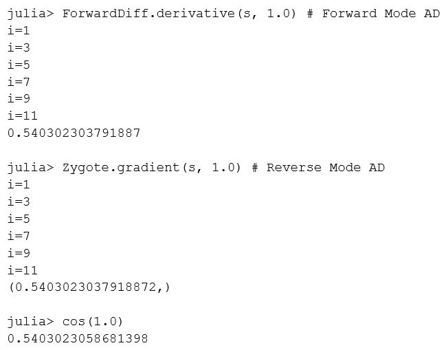
While we could have written the Taylor series for sine more compactly in Julia, we used a loop, a conditional, a print, and function calls to illustrate more complex programs. AD simply works, and that is powerful. Let’s compute the gradient at \(x=1.0\) and verify that it matches \(\cos(1.0)\) (see Figure 2).

\(\partial \textrm{P}\): Differentiating a Trebuchet

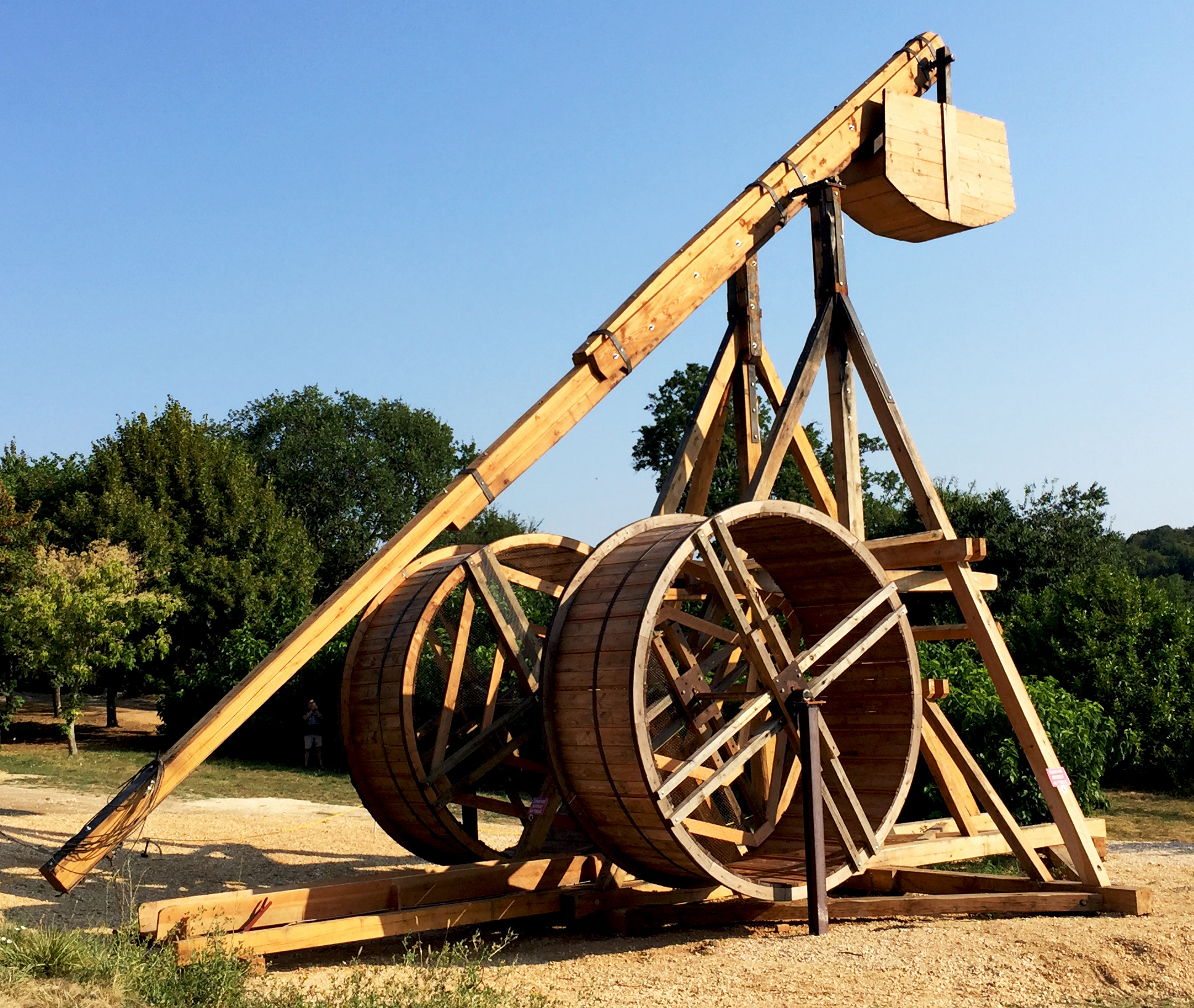
One may wonder if this concept operates successfully on a more complex example. What if we replace tabulated data with a physical model? An example that has captivated attention—perhaps due to its appearance in battle scenes from Game of Thrones—is the trebuchet, a medieval battle catapult (see Figure 3) [1]. We perform \(\partial \textrm{P}\) on the trebuchet, which—despite its deceptively-simple appearance—is a non-trivial system for the purposes of simulation. A differential equation models the distance of a projectile given angle, weight, and wind speed. The human operator can control the projectile’s weight and angle for a set wind speed.

This illustration combines a neural network with the trebuchet’s dynamics (see Figure 4). The network learns the dynamics in a training loop. For a given wind speed and target distance, it generates trebuchet settings (the mass of the counterweight and angle) that we feed into the simulator to calculate the distance. We then compare this distance to our target and backpropagate through the entire chain to adjust the network’s weights. This is where \(\partial \textrm{P}\) arises. The training is quick because we have expressed exactly what we want from the model in a fully-differentiable way; the model is trained within a few minutes on a laptop with randomly-generated data. Compared to solving the inverse problem of aiming the trebuchet by conducting parameter estimation via gradient descent (which takes 100 milliseconds), the neural network (five microseconds) is 20,000 times faster. The Trebuchet.jl repository contains all the necessary code and examples.

The DiffEqFlux.jl project, which further explores many of the ideas in neural ODEs, is also noteworthy. For example, it allows use of an ODE as a layer in a neural network and provides a general framework for combining Julia’s ODE capabilities with neural networks.

Leading institutions like Stanford University; the University of California, Berkeley; and the Massachusetts Institute of Technology continue to utilize Julia for both research and teaching in introductory and advanced courses. We hope our new \(\partial \textrm{P}\) capabilities will help researchers combine ideas in machine learning with those in science and engineering, and ultimately lead to novel breakthroughs.

¹ As 2018 Turing Award winner Yann LeCun said, “Deep learning est mort! Vive differentiable programming.”

Jeff Bezanson, Stefan Karpinski, and Viral B. Shah—creators of the Julia Language—received the James H. Wilkinson Prize for Numerical Software at the 2019 SIAM Conference on Computational Science and Engineering, which took place earlier this year in Spokane, Wash. The prize recognized Julia as “an innovative environment for the creation of high-performance tools that enable the analysis and solution of computational science problems.”

References

[1] Innes, M., Joy, N.M., & Karmali, T. (2019). Differentiable Control Programs. The Flux Machine Learning Library. Retrieved from https://fluxml.ai/2019/03/05/dp-vs-rl.html.
[2] Rackauckas, C. (2019). The Essential Tools of Scientific Machine Learning (Scientific ML). The Winnower 6:e156631.13064. Retrieved from https://thewinnower.com/papers/25359-the-essential-tools-of-scientific-machine-learning-scientific-ml. 

Further Reading

- Bezanson, J., Edelman, A., Karpinski, S., & Shah, V.B. (2017). Julia: A fresh approach to numerical computing. SIAM Rev., 59(1), 65-98. 
- Innes, M. (2019). What is Differentiable Programming? The Flux Machine Learning Library. Retrieved from https://fluxml.ai/2019/02/07/what-is-differentiable-programming.html.
- Rackauckas, C., Innes, M., Ma, Y., Bettencourt, J., White, L., & Dixit, V. (2019). DiffEqFlux. Jl
– A Julia Library for Neural Differential Equations. Preprint, arXiv:1902.02376.