Simply on Maupertuis’ Principle

More than a century after the discovery of Maupertuis’ principle, Jacobi wrote that “This principle is presented incomprehensibly, in my view, in almost all textbooks, including the best ones, such as those by Poisson, Lagrange and Laplace”¹ [1].

In its simplest form, Maupertuis’ principle states a remarkable fact: The trajectory \(\gamma_{\textrm{actual}}\) of a point mass with a prescribed energy \(E\) that flies in a potential force field is a minimizer² of \(\int_\gamma v\;ds\) among all other paths \(\gamma\) that share endpoints with \(\gamma_{\textrm{actual}}.\) Here, \(v\) is the speed as a function of position that is determined when energy \(E\) is prescribed, and \(s\) is the arc length along the path.³

In other words, trajectories with prescribed energy are geodesics in the (Jacobi) metric \(vds.\)

Deriving Maupertuis’ Principle

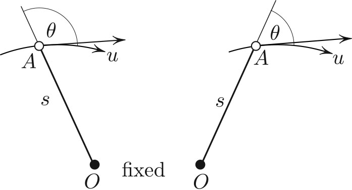
A key part of the explanation lies in a simple geometrical fact illustrated in Figure 1: the distance from a fixed point to a moving point changes at the rate

\[\frac{ds}{du} = \cos \theta, \tag1\]

where the meaning of terms and the reason for \((1)\) are explained in the caption.

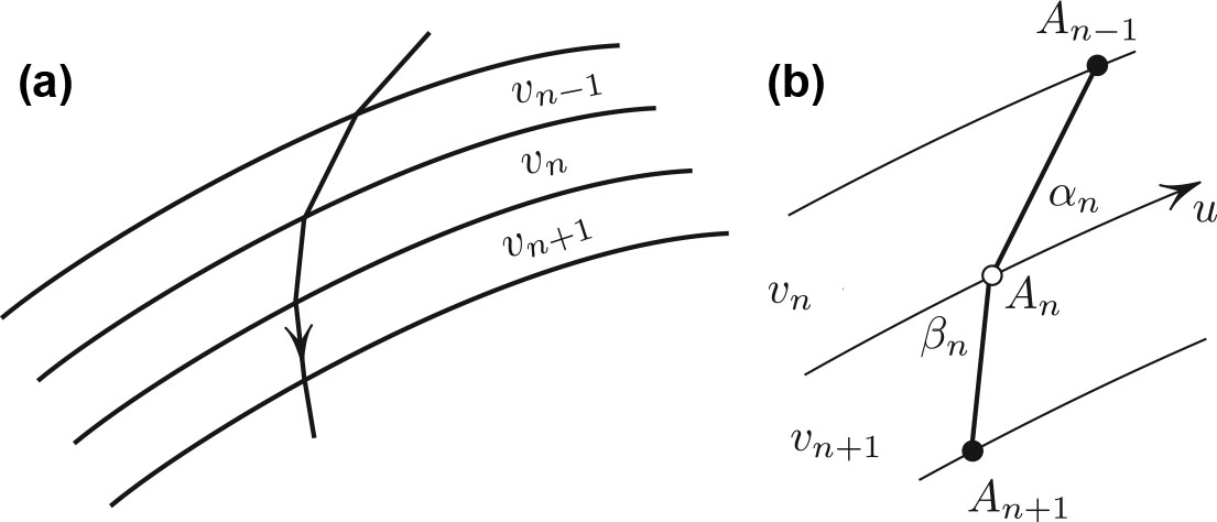
For future reference, \(ds/du<0\) if \(\theta\) is obtuse (see Figure 1). Let us now discretize the potential by replacing it with constant in strips between neighboring level curves (see Figure 2). The particle’s speed \(v_n\) is constant throughout the \(n\)th strip; it is known because the particle’s total energy \(E\) is prescribed. Upon crossing each level curve of the potential, the speed changes in a jump. Crucially, however, the tangential component of the speed does not change (see Figure 2b):

\[v_{n+1} \cos\beta_n - v_n \cos \alpha_n =0. \tag2\]

I claim that \((2)\) amounts to saying that action is stationary for our trajectory. Indeed, let us fix points \(A_{n\pm1}\) and allow \(A_n\) to vary along its level curve, where arc length parameter \(u=0\) corresponds to \(A_n\)’s unperturbed position. According to \((1),\) the lengths \(s_n=A_{n-1}A_n\) and \(s_{n+1}=A_nA_{n+1}\) satisfy at \(u=0:\)

\[\frac{ds_n}{du} = - \cos \alpha_n, \quad \frac{ds_{n+1}}{du} = \cos \beta_n.\]

We can thus rewrite Newton’s law \((2)\) as    

\[\frac{d}{du} \bigl(  v_{n }  s_{n }+ v_{n+1}  s_{n+1}  \bigl)=0 \quad \textrm{at} \quad u=0. \tag3\]

Since this holds for all points of the trajectory, we conclude that the sum \(\sum_{n=0}^N v_ns_n\) is stationary. This sum is an approximation of the action integral \(\int v \; ds,\) thus completing the explanation of Maupertuis’ principle.

To summarize, we only used three facts: (i) energy conservation, which determines \(v_n;\) (ii) a consequence \((2)\) of Newton’s law; and (iii) a simple geometrical observation \((1)\).

Some History

Maupertuis’ principle was discovered by Leibniz around 1707 and published by Euler around 1744, the same year that Maupertuis’ paper appeared [2]. In this paper, Maupertuis considered the refraction of light rays that cross the interface between air and water. He assumed that the light in the air moves more slowly⁴ since \(v_{\rm air}< v_{\rm water}\) and stated—relying on a metaphysical argument—that the rays minimize the action

\[v_{\rm air} s_{\rm air}+ v_{\rm water}v_{\rm water}. \tag4\]

From this assumption, Maupertuis derived the law of refraction

\[v_{\rm air} \sin  \alpha _{\rm air} = v_{\rm water}\sin  \alpha _{\rm air},\]

where \(\alpha\) are the angles with the normal to the interface. This answer would have been correct had velocities been replaced by their reciprocals:

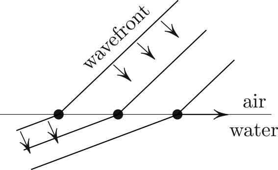
\[\frac{v_{\rm air}}{\sin  \alpha _{\rm air}} = \frac{v_{\rm water}}{\sin  \alpha _{\rm water}}. \tag5\]

I wrote Snell’s law in a slightly unconventional way by putting velocities in the numerator because both sides of \((5)\) have a direct physical meaning, as stated in the caption of Figure 3. Snell’s law is a consequence of the fact that the wavefront only touches the surface at one point at each moment. Both sides of \((5)\) are different expressions of the same thing.

¹ The actual quote is “Dies Princip wird fast in allen Lehrbüchern, auch in den besten, in denen von Poisson, Lagrange und Laplace, so dargestellt, dass es nach meiner Ansicht nicht zu verstehen ist.”

² Or more precisely, makes critical. The trajectory minimizes if it is short enough, i.e., if there are no two conjugate points on this segment of the trajectory.

³ So that \(v = \sqrt{2(E-U)/m}\), where the potential energy \(U\) is the function of position.

⁴ Contrary to what Fermat and Huygens believed several decades earlier.

The figures in this article were provided by the author.

References
[1] Jacobi, C.G.J. (1866). Vorlesungen über dynamik. Berlin, Germany: Druck und Verlag von Georg Reimer.
[2] De Maupertuis, P.L.M. (1744). Accord between different laws of nature that seemed incompatible. Wikisource. Retrieved from https://en.wikisource.org/wiki/Translation:Accord_between_different_laws_of_Nature_that_seemed_incompatible.