The Functions of Deep Learning

Suppose we draw one of the digits $0,1,\dots ,9$. How does a human recognize which digit it is? That neuroscience question is not answered here. How can a computer recognize which digit it is? This is a machine learning question. Both answers probably begin with the same idea: learn from examples.

So we start with $M$ different images (the training set). An image is a set of $p$ small pixels — or a vector $v=(v_1,\dots ,v_p)$. The component $v_i$ tells us the “grayscale” of the $i$th pixel in the image: how dark or light it is. We now have $M$ images, each with $p$ features: $M$ vectors $v$ in $p$-dimensional space. For every $v$ in that training set, we know the digit it represents.

In a way, we know a function. We have $M$ inputs in ${\mathbf{\text{R}}}^p$, each with an output from $0$ to $9$. But we don’t have a “rule.” We are helpless with a new input. Machine learning proposes to create a rule that succeeds on (most of) the training images. But “succeed” means much more than that: the rule should give the correct digit for a much wider set of test images taken from the same population. This essential requirement is called generalization.

What form shall the rule take? Here we meet the fundamental question. Our first answer might be: $F(v)$ could be a linear function from ${\mathbf{\text{R}}}^p$ to ${\mathbf{\text{R}}}^{10}$ (a $10$ by $p$ matrix). The $10$ outputs would be probabilities of the numbers $0$ to $9$. We would have $10p$ entries and $M$ training samples to get mostly right.

The difficulty is that linearity is far too limited. Artistically, two $0$s could make an $8$. $1$ and $0$ could combine into a handwritten $9$ or possibly a $6$. Images don’t add. Recognizing faces instead of numbers requires a great many pixels — and the input-output rule is nowhere near linear.

Artificial intelligence languished for a generation, waiting for new ideas. There is no claim that the absolute best class of functions has now been found. That class needs to allow a great many parameters (called weights). And it must remain feasible to compute all those weights (in a reasonable time) from knowledge of the training set.

The choice that has succeeded beyond expectation—and transformed shallow learning into deep learning—is continuous piecewise linear (CPL) functions. Linear for simplicity, continuous to model an unknown but reasonable rule, and piecewise to achieve the nonlinearity that is an absolute requirement for real images and data.

This leaves the crucial question of computability. What parameters will quickly describe a large family of CPL functions? Linear finite elements start with a triangular mesh. But specifying many individual nodes in ${\mathbf{\text{R}}}^p$ is expensive. It would be better if those nodes are the intersections of a smaller number of lines (or hyperplanes). Please note that a regular grid is too simple.

Figure 1 is a first construction of a piecewise linear function of the data vector $v$. Choose a matrix $A$ and vector $b$. Then set to $0$ (this is the nonlinear step) all negative components of $Av+b$. Then multiply by a matrix $C$ to produce the output $w=F(v)=C(Av+b{)}_{+}$. That vector $(Av+b{)}_{+}$ forms a "hidden layer" between the input $v$ and the output $w$.

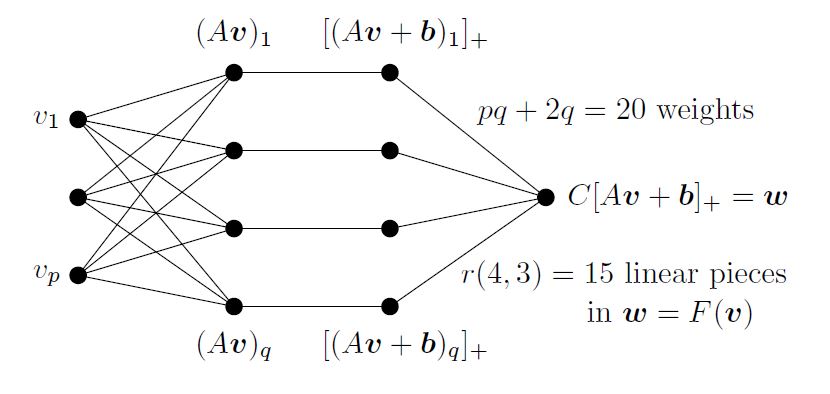
The nonlinear function called $\text{ReLU}(x)=x_{+}=\text{max}(x,0)$ was originally smoothed into a logistic curve like $1/(1+e^{-x})$. It was reasonable to think that continuous derivatives would help in optimizing the weights $A$, $b$, $C$. That proved to be wrong.

The graph of each component of $(Av+b{)}_{+}$ has two half-planes (one is flat, from the $0$s where $Av+b$ s negative). If $A$ is $q$ by $p$, the input space ${\mathbf{\text{R}}}^p$ is sliced by $q$ hyperplanes into $r$ pieces. We can count those pieces! This measures the “expressivity” of the overall function $F(v)$. The formula from combinatorics is

$$r(q,p)=\left(\begin{array}{c}q\\ 0\end{array}\right)+\left(\begin{array}{c}q\\ 1\end{array}\right)+\cdots +\left(\begin{array}{c}q\\ p\end{array}\right).$$

This number gives an impression of the graph of $F$. But our function is not yet sufficiently expressive, and one more idea is needed.

Here is the indispensable ingredient in the learning function $F$. The best way to create complex functions from simple functions is by composition. Each $F_i$ is linear (or affine), followed by the nonlinear $\text{ReLU}:F_i(v)=(A_{i}v+b_i{)}_{+}$. Their composition is $F(v)=F_L(F_{L-1}(\dots F_2(F_1(v))))$. We now have $L-1$ hidden layers before the final output layer. The network becomes deeper as $L$ increases. That depth can grow quickly for convolutional nets (with banded Toeplitz matrices $A$).

The great optimization problem of deep learning is to compute weights $A_i$ and $b_i$ that will make the outputs $F(v)$ nearly correct — close to the digit $w(v)$ that the image $v$ represents. This problem of minimizing some measure of $F(v)-w(v)$ is solved by following a gradient downhill. The gradient of this complicated function is computed by backpropagation: the workhorse of deep learning that executes the chain rule.

A historic competition in 2012 was to identify the 1.2 million images collected in ImageNet. The breakthrough neural network in AlexNet had 60 million weights in eight layers. Its accuracy (after five days of stochastic gradient descent) cut in half the next best error rate. Deep learning had arrived.

Our goal here was to identify continuous piecewise linear functions as powerful approximators. That family is also convenient — closed under addition and maximization and composition. The magic is that the learning function $F(A_i,b_i,v)$ gives accurate results on images $v$ that $F$ has never seen.

This article is published with very light edits.