The Golden Ratio for Cortisol Replacement

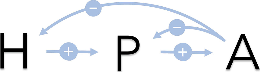
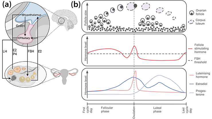
Cortisol, one of the body’s main stress hormones, is primarily responsible for glucose metabolism and immune system regulation. The hypothalamus-pituitary-adrenal (HPA) axis regulates the levels of cortisol in the body (see Figure 1) [4]. Individuals with primary adrenal insufficiency (PAI) are unable to produce a sufficient quantity of cortisol, leading to symptoms such as weight loss, muscle weakness, and low blood pressure [1]. PAI treatment typically involves the use of synthetic cortisol—delivered via continuous intravenous (IV) infusion, repeated IV bolus injection, or in the form of a tablet—to replace what the body cannot make. But since both the quantity and method of treatment affect the resulting levels of hormone in the blood, the optimization of cortisol replacement for individual patients is a complex task. By mathematically modeling the HPA axis, we aim to simulate various treatment regimens to enable the prediction of different (optimal) strategies.

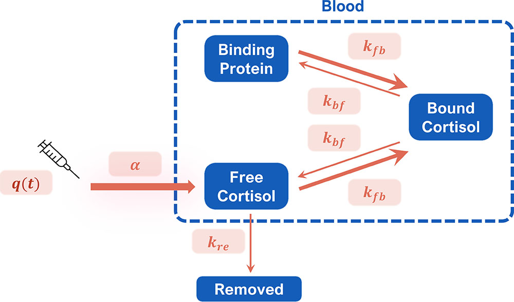
We begin with a single-compartment pharmacokinetic model that builds upon an existing model [3] to estimate concentrations of cortisol in different parts of the body (see Figure 2). Free cortisol—in the form of hydrocortisone—is administered into the blood, where it can bind to proteins or be removed (i.e., metabolized or excreted) from the system. We can write this model with mathematical equations that represent the change in the levels of free cortisol and binding protein over time (derivatives with respect to \(t\)):

\[\frac{dF_f}{dt}= \alpha q(t) - k_{fb}F_fB + k_{bf}F_b - k_{re}F_f, \tag1\]

\[\frac{dB}{dt}= - k_{fb}F_fB + k_{bf}F_b, \tag2\]

\[\frac{dF_b}{dt}= + k_{fb}F_fB - k_{bf}F_b. \tag3\]

The key considerations that underly this model are (i) the binding protein (corticosteroid-binding globulin)’s high affinity for free cortisol and (ii) the fact that only free cortisol can be removed from the system. The following initial conditions are also present:

\[F_f(0)=0, \;\;\;\; B(0) = B_0,\]

\[F_b(0) = 0, \tag4\]

where \(B_0\) is the physiological level of binding protein. We assume that the amount of cortisol in a patient with adrenal insufficiency is negligible (a simplification that we will further consider in the future). Here, \(q(t)\) is a known input of the drug dose. We have three state variables—free cortisol \((F_f)\), bound cortisol \((F_b)\), and unoccupied binding protein \((B)\)—as well as five unknown parameters \((\alpha,\) \(k_{fb},\) \(k_{bf},\) \(k_{re},\) and \(B_0)\) that we wish to fit via patient data. By eliminating bound cortisol, we can reduce the model to a system of two ordinary differential equations (ODEs):

\[\frac{dF_f}{dt}=\alpha q(t)- k_{fb}F_fB + k_{bf}(B_0-B) - k_{re}F_f, \tag5\]

\[\frac{dB}{dt}= - k_{fb}F_fB + k_{bf}(B_0-B). \tag6\]

Temporal Evolution of Cortisol

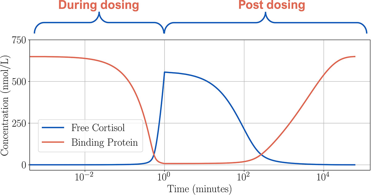
Solving the ODE model reveals the way in which the free cortisol and binding protein concentrations change throughout a single high-dose period (see Figure 3). To do so, we model an IV bolus as a high dose that is delivered continuously over a one-minute period, i.e.,

\[ q(t) = \begin{cases}
                q, & 0\leq t\leq1\\
                0, & 1<t. 
            \end{cases} \tag7\]

During dosing, the binding protein and cortisol quickly bind, thereby reducing the level of free cortisol. In this high-dose case, the binding protein is almost completely saturated by the end of the dosing period; once dosing concludes, free cortisol is eliminated and removed from the system. Binding and unbinding occur continuously, which leads to a slow increase in the binding protein. Eventually, all cortisol is removed.

Rational Model Simplification

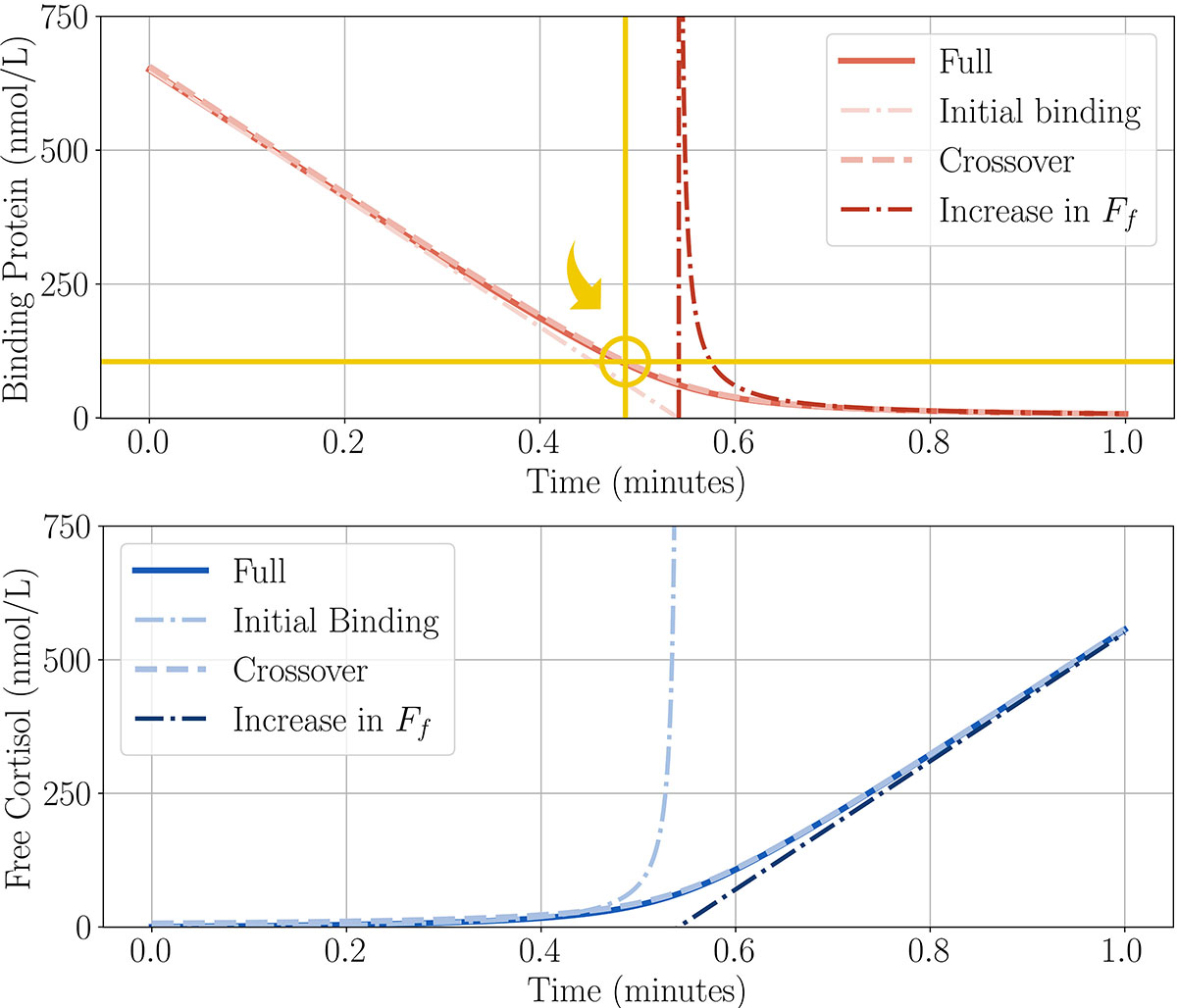
Based on small amounts of empirical data, we assume that binding is the fastest process in the system, followed by unbinding [2]. These two processes each occur on much shorter timescales than the dosing period of one minute, which is still significantly faster than the removal rate (see Figure 4). This insight allows us to simplify the model and will facilitate parameter estimation when we ultimately fit our model to data, as it can reduce and simplify the equations we want to solve and/or reduce the number of unknown parameters we seek to estimate.

A Fun Aside: The Golden Ratio Emerges

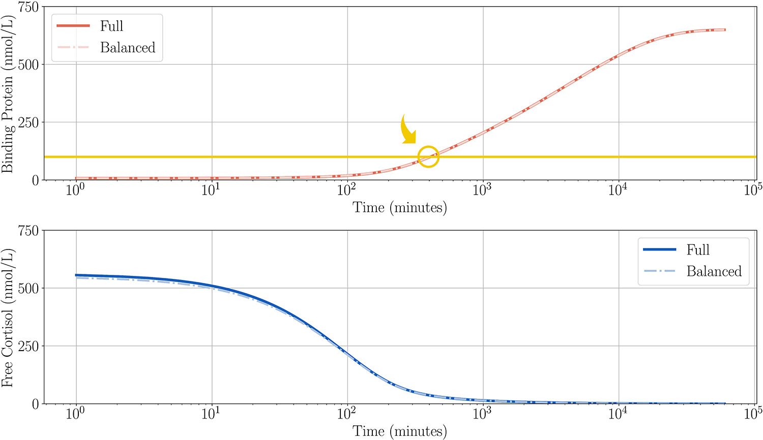
We now break the full solution into three different regions as free cortisol and the binding protein interact. By separating the rates, we see that binding is the dominant process in the dosing period. Initially, the binding protein is saturated by incoming free cortisol (see “Initial Binding” in Figure 5). Once the protein is mostly saturated, the amount of free cortisol rises steadily (see “Increase in \(F_f\)" in Figure 5). We want to find a combination of solutions that will match the entire dosing period, so we look for a third crossover region to bridge the gap between the other two solutions (see “Crossover” in Figure 5). Within this region, we see that the level of unoccupied binding protein crosses through a value that is proportional to the golden ratio (circled in gold in Figure 5). In dimensional variables, 

\[B = B_0 \delta^\frac{1}{2} \left({\color{gold}{\frac{1+\sqrt{5}}{2}}}\right) \quad \text{at} \quad t = \frac{B_0\tau}{\alpha D}\left(1-\left(\frac{k_{bf}}{k_{fb}B_0}\right)^\frac{1}{2}\right).\]

After delivery of the dose, we can reduce the model to a single equation that describes the remainder of the time (see Figure 6). We begin by defining a new variable \(x\) for the difference between the two variables \((x=F_f-B)\). This new variable allows us to eliminate \(F_f\) from the system and obtain a novel pair of ODEs with one slow and one fast variable. From this new system, we then take an asymptotic expansion and equate coefficients to find an ODE for the slow manifold solution of \(x\). The resulting single equation describes the unbinding and the gradual removal of cortisol, with protein returning to pre-dosing levels. Notably, the golden ratio appears again as the binding protein increases:

\[B = B_0\delta^\frac{1}{2}\left(1-\frac{\delta^\frac{1}{2}}{\sqrt{5}}\right)\left({\color{gold}{\frac{1+\sqrt{5}}{2}}}\right).\]

With this approach, we aim to fit the simplified model to patient response data and estimate model parameters. The model reductions allow us to solve the system much more quickly, which will assist with parameter inference. In the long term, we hope to test different treatment strategies to determine what works best for a particular individual. This effort is particularly important for patients who undergo other stressors, as their dosing amounts may consequently require alterations.

Rosie Evans delivered a contributed presentation on this research at the 2023 SIAM Conference on Applications of Dynamical Systems (DS23), which took place in Portland, Ore., in May 2023. She received funding to attend DS23 through a SIAM Student Travel Award. To learn more about Student Travel Awards and submit an application, visit the online page. 

SIAM Student Travel Awards are made possible in part by the generous support of our community. To make a gift to the Student Travel Fund, visit the SIAM website. 

Acknowledgements: The authors would like to thank Wiebke Arlt and her team at the University of Birmingham for providing the data around which this work is based.

References
[1] Charmandari, E., Nicolaides, N.C., & Chrousos, G.P. (2014). Adrenal insufficiency. Lancet, 383(9935), 2152-2167.
[2] Picard-Hagen, N., Gayrard, V., Alvinerie, M., Smeyers, H., Ricou, R., Bousquet-Melou, A., & Toutain, P.L. (2001). A nonlabeled method to evaluate cortisol production rate by modeling plasma CBG-free cortisol disposition. Am. J. Physiol. Endocrinol. Metab., 281(5), E946-E956.
[3] Smith, D.J., Prete, A., Taylor, A.E., Karavitaki, N., & Arlt, W. (2020). Modelling oral adrenal cortisol support. Preprint, arXiv:2006.00043.
[4] Zavala, E., Wedgwood, K.C.A., Voliotis, M., Tabak, J., Spiga, F., Lightman, S.L., & Tsaneva-Atanasova, K. (2019). Mathematical modelling of endocrine systems. Trends Endocrinol. Metab., 30(4), 244-257.