The Optimality of Bayes’ Theorem

Inverse problems are pervasive in scientific discovery and decision-making for complex, natural, engineered, and social systems. They are perhaps the most popular mathematical approach for enabling predictive scientific simulations that integrate observational/experimental data, mathematical models, and prior knowledge. While indirect data provide valuable information about unknown parameters and the physical problem itself, such data are typically limited and therefore unable to sufficiently infer the parameters. Conversely, the prior encodes a priori knowledge about the parameters and its bias is thus unavoidable.

Of the many frameworks that facilitate uncertainty quantification in inverse solutions, the Bayesian paradigm is perhaps the most popular.¹ The Bayesian approach combines prior knowledge (via prior distribution of the parameters) with observational data (via the likelihood) to produce the posterior probability distribution as the inverse solution. The following two-part question hence arises: Is this method of using observed information from data the best way to update the prior distribution? If so, in what sense? Answering these queries yields insight into Bayes’ theorem and brings to light meaningful interpretations that are otherwise hidden.

Here we utilize three different perspectives—two from information theory and one from the duality of variational inference—to show that Bayes’ theorem is in fact an optimal way to blend prior and observational information. To that end, let us use \(\mathbf{m}\) to denote the unknown parameter of interest, \(\pi_\textrm{prior}(\mathbf{m})\) for the prior density (or distribution), \(\pi_\textrm{like}(\mathbf{d}|\mathbf{m})\) for the likelihood of \(\mathbf{m}\) given observable data \(\mathbf{d}\), and \(\pi_\textrm{post}(\mathbf{m}|\mathbf{d})\) for the posterior density. Every student of the Bayesian inference framework presumably knows that according to conditional probability [1], Bayes’ formula—the sole result of Bayes’ theorem—reads

\[\pi_\textrm{post}(\mathbf{m}|\mathbf{d}):=\frac{\pi_\textrm{like}(\mathbf{d}|\mathbf{m})\times\pi_\textrm{prior}(\mathbf{m})}{\mathbb{E}_{{\pi}_\textrm{prior}}[\pi_\textrm{like}(\mathbf{d}|\mathbf{m})]},\tag1\] 

where \(\mathbb{E}_{{\pi}_\textrm{prior}}[\cdot]\) denotes the expectation under the prior distribution. Bayes’ formula \((1)\) provides a simple formula for the posterior as the product of the prior and likelihood. Indeed, it is so simple that deep insights are perhaps neither necessary nor possible. In fact, most researchers likely never wonder why such a simple framework is so effective for many statistical inverse problems in engineering and the sciences.

Calculus of variations tells us that if an optimizer for some objective functional exists, it has to satisfy the first-order optimality condition (equation) that indicates that the first variation of the objective functional at the optimum must vanish. The equation form of Bayes’ formula \((1)\) triggers our curiosity and prompts us to wonder whether Bayes’ formula is the first-order optimality condition of some objective functional. To approach this question, we note that the prior encodes our prior knowledge/belief before we see the data. From the point of view of information theory, we should elicit the prior so that its discrepancy relative to the updated distribution \(\rho(\mathbf{m})\) (to be found) is as small as possible. That is, if we believe that our prior is meaningful, the information that we gain from the data in \(\rho(\mathbf{m})\) should not be significant. The relative loss or gain between two probability densities is precisely captured by the relative entropy, also known as the Kullback-Leibler (KL) divergence [3]: \(D_\textrm{KL}(\rho|\pi_\textrm{prior}):=\)\(\mathbb{E}_\rho[\log(\frac{\rho(\mathbf{m})}{\pi_\textrm{prior}(\mathbf{m})})]\). When the updated distribution \(\rho(\mathbf{m})\) is identical to the prior \(\pi_\textrm{prior}(\mathbf{m})\), the KL divergence is zero — i.e., the prior is perfect. But when \(\rho(\mathbf{m})\) deviates from the prior \(\pi_\textrm{prior}(\mathbf{m})\)—e.g., when the data provides additional information or strengthens some information in the prior—the KL divergence is positive.

Since the observational data \(\mathbf{d}\) is the other piece of information in the posterior’s construction, we wish to match the data as well as possible while avoiding overfitting. One way to do so is to look for \(\rho(\mathbf{m})\) that minimizes \(-\mathbb{E}[\log(\pi_\textrm{like}(\mathbf{d}|\mathbf{m}))]\), which is a generalized mean squared error (MSE) that comes from using the updated distribution to predict the data.

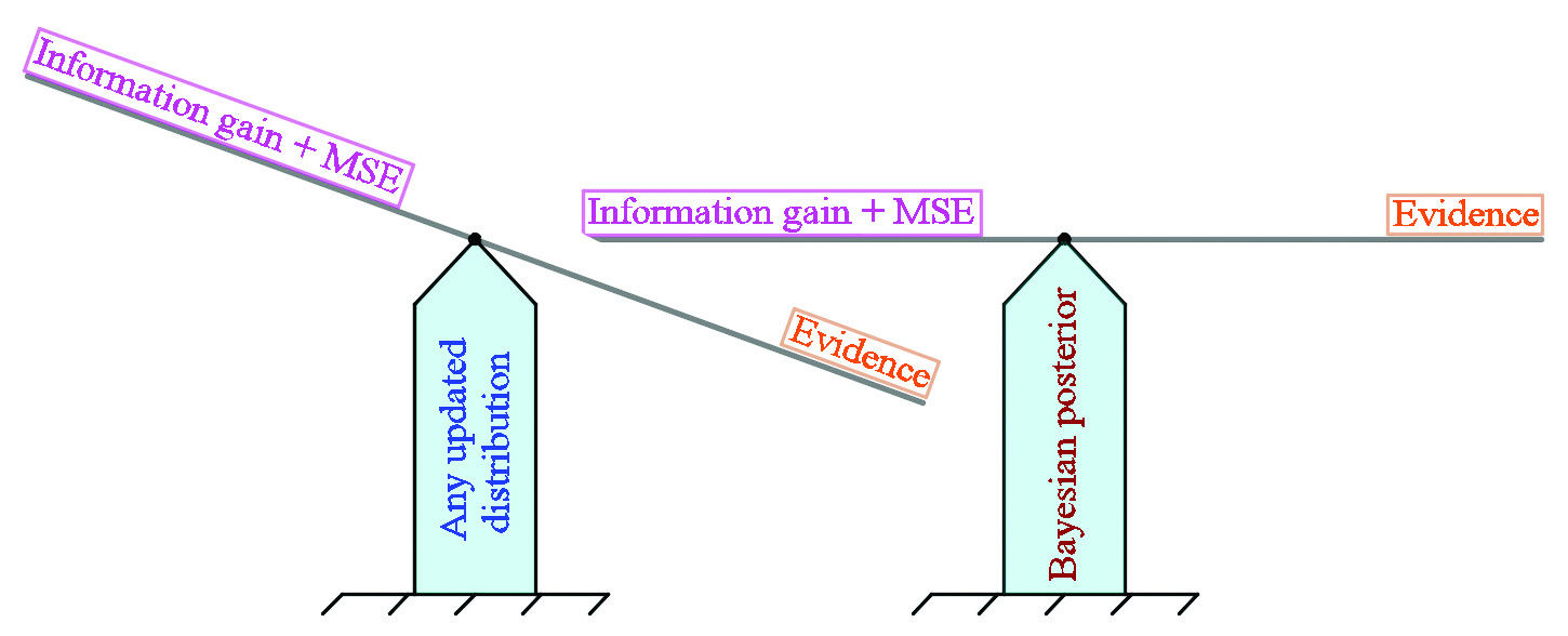
At this point, we see that a competition exists between the prior knowledge and the information from the data in terms of constructing the updated distribution. On the one hand, the updated distribution should be close to the prior if we believe that the prior is the best within our subjective elicitation. On the other hand, the updated distribution should be constructed in such a way that the data is matched well under that distribution. We argue that the optimal updated distribution should compromise these two sources of information so that it captures as much of the limited information from the data as possible while also resembling the prior. We can construct such a distribution by simultaneously minimizing the KL divergence and MSE (see Figure 1 for a demonstration) [2], i.e.,

\[\underset{\rho(\mathbf{m})}\min D_\textrm{KL}(\rho|\pi_\textrm{prior})-\mathbb{E}_\rho[\log(\pi_\textrm{like})].\tag2\]

The beauty here is that the optimization problem \((2)\) is convex, its first-order optimality condition is precisely Bayes’ formula \((1)\), and its unique updated distribution is exactly Bayes’ posterior \(\pi_\textrm{post}(\mathbf{m}|\mathbf{d})\).

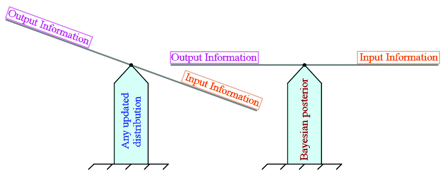
We can also achieve the optimality of Bayes’ formula \((1)\) from an information conservation principle [5]. In this approach,² we divide the information—with respect to the updated distribution \(\rho(\mathbf{m})\)—into the input information \(\mathbb{E}_\rho[\log\pi_\textrm{prior}(\mathbf{m})+\log\pi_\textrm{like}(\mathbf{d}|\mathbf{m})]\) that is provided by the prior \(\rho(\mathbf{m})\) and likelihood \(\pi_\textrm{like}(\mathbf{d}|\mathbf{m})\), and the output information \(\mathbb{E}_\rho[\log\rho(\mathbf{m})+\log\mathbb{E}_{\pi_\textrm{prior}}[\pi_\textrm{like}(\mathbf{d}|\mathbf{m})]]\) that is provided by the updated distribution \(\rho(\mathbf{m})\) and evidence \(\mathbb{E}_{\pi_\textrm{prior}}[\pi_\textrm{like}(\mathbf{d}|\mathbf{m})]\). The optimal updated distribution is the one that minimizes the difference between the output and input information — it is exactly Bayes’ posterior \(\pi_\textrm{post}(\mathbf{m})\), at which the difference is zero [5]. In other words, Bayes’ posterior is the unique distribution that satisfies the information conservation principle (see Figure 2 for a demonstration).

Next, we show that the optimality of Bayes’ formula \((1)\) is also apparent from a duality formulation of variational inference [4]. Under mild conditions on \(\pi_\textrm{prior}(\mathbf{m})\), \(\rho(\mathbf{m})\), and a large class of functions \(f(\mathbf{m})\), the following inequality holds true:

\[-\log\mathbb{E}_{\pi_\textrm{prior}}[e^{f(\mathbf{m})}]\le\mathbb{E}_\rho[-f(\mathbf{m})]+D_\textrm{KL}(\rho|\pi_\textrm{prior}).\]

The equality occurs when the right-hand side of the formula attains its minimum and the unique optimizer \(\rho(\mathbf{m})\) satisfies \(\rho(\mathbf{m})\times\mathbb{E}_{\pi_\textrm{prior}}[e^{f(\mathbf{m})}]=e^{f(\mathbf{m})}\times\pi_\textrm{prior}(\mathbf{m})\). Taking \(f(\mathbf{m})=\log(\pi_\textrm{like}(\mathbf{d}|\mathbf{m}))\), we immediately conclude that the optimal \( \rho(\mathbf{m})\) is the Bayes’ posterior \(\pi_\textrm{post}(\mathbf{m})\). In this case, the right-hand side is exactly the objective functional \((2)\). The objective functional’s minimum is the negative log evidence (the left-hand side of the formula); this is achieved only at Bayes’ posterior (see Figure 1).

Here we show that Bayes’ formula has a firm foundation in optimization. In particular, one can view the formula as the first-order optimality condition for three different yet related optimization problems: (i) simultaneous minimization of the information gain from the prior and the MSE of the data, (ii) minimization of the output and input information discrepancy, and (iii) minimization of the upper bound of a variational inference problem. This material yields additional insight into the Bayesian inference framework and paves the way for the development of optimization approaches for Bayesian computations.

¹A Google search for “Bayes’ theorem” returns 7,510,000 results. 

²The approach in [2] was discovered independently of [5]. 

Acknowledgments: This work was partially funded by the National Science Foundation (NSF) awards NSF-1808576 and NSF-CAREER-1845799; the Defense Threat Reduction Agency (DTRA) award DTRA- M1802962; the Department of Energy award DE-SC0018147; the 2020 ConTex Award; and the 2018 UT-Portugal CoLab award.

References 

[1] Bayes, T. (1763). LII. An essay towards solving a problem in the doctrine of chances. By the late Rev. Mr. Bayes, F.R.S. communicated by Mr. Price, in a letter to John Canton, A.M.F.R.S. Philos. Trans. Royal Soc. Lond., 53, 370-418. 
[2] Bui-Thanh, T., & Ghattas, O. (2015). Bayes is optimal (Technical report ICES-15-04). Austin, TX: The Oden Institute for Computational Engineering and Sciences.
[3] Jaynes, E.T. (2003). In Bretthorst, G.L. (Ed.), Probability theory: The logic of science. Cambridge, U.K.: Cambridge University Press.
[4] Massart, P. (2003). Concentration inequalities and model selection. Ecole d’eté de probabilités de saint-flour xxxiii. In Lecture notes in mathematics (Vol. 1896). Berlin: Springer-Verlag. 
[5] Zellner, A. (1988). Optimal information processing and Bayes’s theorem. Am. Stat., 42(4), 278-280.