The Rational Krylov Toolbox: Nonlinear Rational Approximation

In the April 2022 issue of SIAM News, I provided a brief introduction to rational Krylov methods—a critical tool in the field of scientific computing—and discussed several applications. Now I focus on the RKFIT method for nonlinear rational approximation, one of the core algorithms in the freely available MATLAB Rational Krylov Toolbox (RKToolbox). The toolbox comprises an extensive collection of examples that users can explore and modify; here they are printed in typewriter font for easy identification.

Nonlinear Rational Approximation

The purpose of RKFIT is to solve nonlinear least-squares problems

\[\| Fb - r(A)b \|_2 \to \min_r,\tag1\]

where \(A\) and \(F\) are given square matrices of the same size and \(b\) is a given vector of compatible size. In the simplest case, the minimization in \((1)\) occurs over all rational functions \(r\) of degree \(m\) (i.e., quotients \(r=p/q\) of two polynomials of degree \(m\)). This is a nonconvex minimization problem that may be ill posed, meaning that we can generally only ask for a solution that makes the left side of \((1)\) “small.”

The formulation \((1)\) contains several familiar special cases, including rational approximation on a discrete set when both \(A\) and \(F\) are diagonal matrices, or multi-point Padé approximation when \(A\) has nontrivial Jordan blocks. In many applications, \(F=f(A)\) is a complicated matrix function of \(A\); we thus aim to compute \(r\) without resorting to \(A\)'s eigenvalues or other spectral information. RKFIT achieves this objective by iteratively transforming the matrices in a rational Arnoldi decomposition and solving least-squares problems with orthonormal rational Krylov bases; more details are available elsewhere [1, 3].

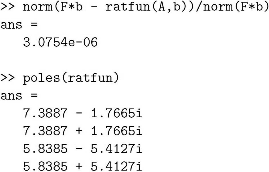
The use of RKFIT in the RKToolbox is straightforward; Figure 1 presents a basic example. This code computes a degree-4 rational function \(r\) such that \(r(A)b \approx Fb\) for the nonnormal Grcar matrix \(A\), which is a popular test matrix in numerical analysis. The computed function is represented by an RKFUN object called ratfun that users can incorporate in further computations. Figure 2 checks the relative error \(\|Fb - r(A)b\|_2/\|Fb\|_2\) and displays the four poles of \(r\).

RKFIT has a number of optional functionalities and parameters that individuals can list by typing help rkfit. For instance, instead of providing F as a dense matrix like in our basic example, it is typically more efficient to provide a function handle for the computation of matrix-vector products; it is also possible to enforce stable poles (param.stable). The RKToolbox contains several RKFIT-related examples, two of which I will discuss in some detail.

Exponential Integration

Linear initial value problems such as \(u'+A u = 0\), \(u(0)=b\)—where \(A\) is a large sparse matrix—arise in many applications. In the RKToolbox demonstration at example_expint.hmtl, we are concerned with the efficient solution of this problem with uniform accuracy over a given time interval, say \([T_0,T_1]\). The solution, which is given as \(u(t) = e^{-At}b\),  can conveniently be approximated by a family of rational functions in partial fraction form:

\[r^{(t)}(A)b = \sum_{i=1}^m \alpha_i(t) ( \xi_i I - A)^{-1}b \approx e^{-At}b.\]

Note that the poles \(\xi_i\) of \(r^{(t)}\) are independent of \(t\) and the evaluation of \(r^{(t)}(A)b\) hence requires the solution of \(m\) shifted linear systems \((\xi_i I - A)x_i = b\), which are independent of the number of time points \(t\) for which we want to evaluate. Furthermore, all of these linear systems are decoupled and can be solved in parallel.

A popular approach for obtaining families of such rational approximants is to apply a quadrature discretization to the Cauchy integral formula

\[e^{-At} = \frac{1}{2\pi \mathrm{i}} \int_\Gamma e^{-\zeta t} (\zeta I - A)^{-1} \mathrm{d}\zeta \]

with an appropriately chosen contour \(\Gamma\) that encloses \(A\)'s eigenvalues [4]. Alternatively, we can run RKFIT to numerically compute a family of rational approximants so that the error \(\|e^{-At}b - r^{(t)}(A)b\|_2\) is uniformly small for all \(t \in [T_0, T_1]\). To that end, RKFIT employs a surrogate approach wherein \(A\) and \(b\) are replaced by a “simpler” matrix \(\widehat A\) and vector \(\hat b\). The surrogate matrix \(\widehat A\) should capture \(A\)'s spectral properties while being easy to compute with. For instance, one could obtain \(\widehat A\) from a coarser discretization if \(A\) arises from the spatial discretization of a differential operator. Figure 3 illustrates an example of this concept [1]. Here, the matrix \(A\) is symmetric positive semidefinite and the time interval of interest is \([T_0,T_1] = [0.1,10]\). 

Figure 3a displays the approximation error of both the original and surrogate problems. The RKFIT family of rational approximants \(r^{(t)}(A)b\) achieves a near-uniform error over the entire time interval. We also compare this approach to a contour integration-based technique that is optimized for a single time parameter \(t=1\), where the poles of the rational function lie on a prescribed contour (see Figure 3b). The contour approach achieves a high accuracy at \(t=1\), but the accuracy deteriorates significantly at other time points.

Compression of Layered Waveguides

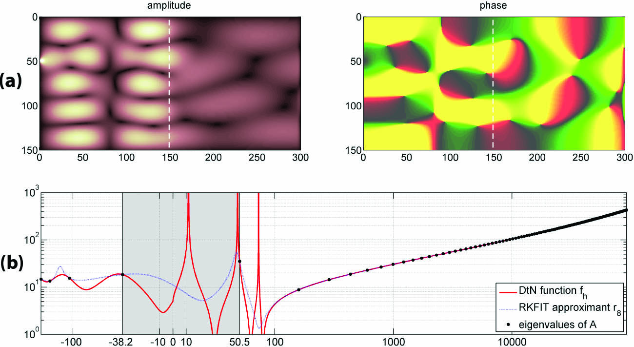
The example at example_ehcompress.html relates to absorbing boundary conditions for wave problems and the optimization of transmission conditions in domain decomposition methods. Consider a two-dimensional waveguide with varying wave number in the horizontal direction (see Figure 4a). Depending on the structure of the layers, the Dirichlet-to-Neumann (DtN) map of this waveguide, \(f(A)\), may be a highly irregular matrix function where \(f\) has many singularities (so-called scattering poles) near \(A\)'s eigenvalues. It is therefore impossible to construct a uniform rational approximant \(r(A)\approx f(A)\) on \(A\)'s spectral region. We recently proposed the computation of a low-order RKFIT approximant \(r(A)b\approx f(A)b\) with a random probing vector \(b\) [2]. The continued fraction form of \(r\) is equivalent to a finite-difference representation of the DtN map; this representation can be appended to an existing discretization as an artificial boundary condition.

An important property of RKFIT approximants is their inherent spectral adaptation. Even though one does not explicitly need \(A\)'s eigenvalues to run RKFIT, the computed approximant will resolve the function \(f\) more accurately in some parts of the spectrum than in others (see Figure 4b). This spectral adaptation effect allows for the construction of finite-difference grids that undercut the Nyquist limit for discretizations of wave problems [2].

Summary

Here I have presented a brief introduction to the RKFIT method for nonlinear rational approximation and discussed two sample applications. The RKToolbox provides some additional RKFIT examples that are related to model order reduction (example_frequency.html and example_iss.html) and graph label propagation (example_digits.html). All figures are courtesy of the author.

References

[1] Berljafa, M., & Güttel, S. (2017). The RKFIT algorithm for nonlinear rational approximation. SIAM J. Sci. Comput., 39(5), A2049-A2071.
[2] Druskin, V., Güttel, S., & Knizhnerman, L. (2022). Model order reduction of layered waveguides via rational Krylov fitting. BIT Numer. Math. To appear. 
[3] Güttel, S. (2022, April 1). The rational Krylov toolbox. SIAM News, 55(3), p. 10.
[4] Trefethen, L.N., Weideman, J.A.C., & Schmelzer, T. (2006). Talbot quadratures and rational approximations. BIT Numer. Math., 46(3), 653-670.