
The Statistical Formalism of Uncertainty Quantification
Since the launch of the SIAM Activity Group on Uncertainty Quantification in 2010, the applied mathematics community has seen an explosion of interest in the topic. Uncertainty quantification (UQ) considers the uncertainties in both the mathematical modeling of processes and the associated data; it is now recognized as an essential component of math modeling.
In 2019, we reviewed the statistical formalism of UQ [2] that was originally introduced in 2001 [9], including the strengths and weaknesses of the formalism and UQ in general. The implementation of this formalism would provide a “gold standard” for UQ—although some might object to the Bayesian formulation—because it would force us to consider all conceivable uncertainties in a given process.
A simpler, more easily deployable Monte Carlo approach to UQ is the ensemble approach. This concept is best illustrated by numerical weather prediction (NWP). For more than 30 years, forecasters have used NWP to sample uncertainties in important variables and compute a number of potential weather trajectories (each of which is a member of the ensemble), revising the ensemble every six hours.
In a sense, statistical formalism and ensemble techniques are actually manifestations of the same idea; given an enormous number of ensemble members and a perfect model, one could reach accountable probabilistic conclusions that are conditioned on current knowledge. In reality, however, operational ensembles tend to have fewer than 100 members, while modern models are imperfect and may contain millions of state variables. Although researchers cannot expect perfect probabilistic conclusions, the ensemble approach provides demonstrably useful information about future real-world weather — even more than 10 days in advance. No approach to UQ can precisely account for structural model error or perform reliably in truly novel conditions, but the coherent deployment of UQ still provides undeniably valuable outcomes. Here, we illustrate the strengths and weaknesses of the statistical formalism and of the ensemble approach to delineate both their successes and remaining challenges. Details about additional approaches to UQ are available in the literature [11].
Some of the most fundamental questions in UQ are (i) How can we provide sufficiently reliable uncertainties? and (ii) How can we assess their reliability a priori? While it is admirable to attempt to account for all possible uncertainties, extrapolating UQ applications to situations that are far from the original scenario is a significant challenge. The ensemble method provides useful uncertainty guidance for weather forecasting, but application to other unobserved situations and untested models—as in climate prediction [10, 12]—makes interpretation similarly tough. Addressing these difficulties is a key research goal in UQ.
![<strong>Figure 1.</strong> Time series of the forces that impact a vehicle’s suspension system as it passes over two potholes. Vertical lines indicate the reference peak locations at which the curves were registered. <strong>1a.</strong> Seven field runs for the pothole 1 region. <strong>1b.</strong> Seven field runs for the pothole 2 region. <strong>1c.</strong> 65 runs of the computer model at pothole 1. <strong>1d.</strong> 65 runs of the computer models at pothole 2. Figure courtesy of [2].](/media/ylan0lyk/figure1.jpg)
Computer Model for a Vehicle Suspension System
Figure 1 depicts a time series of the forces that impact a vehicle’s suspension system as it passes over two potholes in a road. Figures 1a and 1b show seven observed force curves as the vehicle was repeatedly run over the potholes.
A finite element partial differential equation computer model mimics this process, with the goal of replacing pricey field runs in the design of suspension systems with less expensive computer modeling [1]. Figures 1c and 1d illustrate 65 runs of the computer model for 65 differing values of the vector input \(\mathbf{v}=(u_1,u_2,x_1,...,x_7)\). The coordinates of this vector reflect features of the suspension system—such as energy damping (\(u_1\) and \(u_2\)) and suspension stiffness (\(x_i\))—at various locations in the suspension. The computer model was run at various input values because the relevant values for the real vehicle were not precisely known.
UQ seeks to assess the extent to which computer model predictions reflect the real process. One can perform a Bayesian analysis to estimate the discrepancy between the model and reality. Figure 2 shows that the discrepancy for the pothole study is significantly nonzero, especially near time 9. Engineers and designers can use this knowledge to improve the model.
![<strong>Figure 2.</strong> Posterior discrepancy curve estimate (dashed line) and 90 percent confidence bands (solid lines) for the first pothole region. Figure courtesy of [2].](/media/2q1d0s45/figure2.jpg)
Another goal of UQ is to solve an inverse problem to successfully estimate the actual inputs \(\mathbf{v}\). The solid lines in Figure 3 provide the initial prior distribution for the inputs, while the histograms give the final posterior distributions. Furthermore, UQ also aims to use all available information (field runs, computer model runs, and prior distributions) to predict the outcome of a new situation. When a different vehicle (with a different suspension) was repeatedly run over pothole 1, it produced the red curves in Figure 4; this information was initially withheld from the UQ analysts. Instead, they had to predict these curves based on field data for the original vehicle and the 65 computer model runs. By utilizing the full joint distribution of all unknowns, Bayesian analysis yielded the predictions in Figure 4.
The predictions clearly fall within the uncertainty bands for \(t<10\), and the engineers deemed this level of accuracy to be adequate for their purposes. The use of discrepancy in the predictions enabled this successful UQ analysis.
The statistical formalism outlined previously is a natural way to represent the problem at hand. If all of the needed data (field runs and computer model runs) are available and one can accurately conduct probabilistic modeling (specifically, if the Bayesian computation is feasible), then the result is satisfactory. We now turn to five challenges that are associated with UQ.
Challenge 1: Lack of Available Data for Real Scenarios
Engineers often obtain field data of the real process in question (e.g., the suspension system force curves). In many situations, however, the data is incomplete and limited. For instance, scientists only have sparse direct observations of the weather, ocean, and other drivers of climate from the last few hundred years; even satellite observations of a system’s state are far from complete. Weather models are essentially simplified climate models in which many processes are simulated naively or taken as constant. Without a sufficient number of observations, a UQ program that utilizes discrepancy is a nonstarter [7].
Challenge 2: Limited Computer Model Runs and Emulation
Realistic simulation models are often very computationally expensive, which makes the development of an additional approximation—known as an emulator or surrogate—necessary for discrepancy-based UQ analysis. One popular method of emulator construction is via Gaussian processes [5, 6]. Of course, an excellent emulator will reproduce the target model's structural model error, not alleviate it.
In both weather forecasting and climate prediction, ensemble approaches achieve partial UQ by explicitly sampling specific sources of uncertainty. Scientists input sets of different initial conditions, parameter values, and even model structures, then interpret the resulting model runs as a predictive distribution [3]. This approach has proven informative for operational weather forecasting and—more recently—the study of climate model sensitivity [12]. In each case, the relevant prior probability distribution is unknown (assuming that one even exists), the initial input state space is enormous (\(>10^7\)), and hundreds of unknown (and arguably ill-defined) model inputs exist in the form of physical and numerical parameters. In addition, the presence of structural model error—i.e., the model’s equations cannot mimic reality in detail—further complicate the situation [7, 10]. Although the use of ensembles is a major improvement from running one "best" model a single time, it does not provide a full UQ analysis.
![<strong>Figure 3.</strong> Posterior densities of the inputs \(\mathbf{v}\). The solid lines represent the prior densities. Figure courtesy of [2].](/media/5x4lf0zm/figure3.jpg)
Challenge 3: Issues with Model Discrepancy
The acknowledgment of discrepancy in the UQ formalism was undoubtedly a significant conceptual advancement, but the extent to which we can actually evaluate discrepancy is less clear. When researchers build computer models, they must omit certain relevant information. For instance, the mountain ridges in any current climate model are not realistic due to limitations of numerical resolution; precipitation due to orographic effects thus fails to be verisimilar. These types of known neglecteds—which are either handled by an ad hoc process or simply ignored—represent a challenge for formal UQ. Good UQ practice should provide upper bounds on the effect of known neglecteds for all outputs of interest.
The Intergovernmental Panel on Climate Change (IPCC) has long recognized that structural model error will yield uncertainties for which ensemble simulations cannot account [12]. Indeed, the most recent IPCC report employs both model output and expert opinion to obtain quantitative projections that are clearly distinct from (i.e., wider than) the distribution of model runs. One can address certain problems with structural model error—which generally hold in forecasting via nonlinear simulation [10]—by sampling aspects of the dynamics of competing models without explicitly reformulating them [4]. UQ aims to better quantify all of these uncertainties, improve the framework for discussion, and ideally provide decision-relevant probability distributions.
Domain specialists and modelers can often intuit a given model’s ability to successfully track reality up to a certain point, before the occurrence of a “big surprise”: a future event after which reality evolves in a manner that the model cannot shadow. The problem is that we cannot quantify the inconceivable, regardless of how obvious it may seem after the fact. Nevertheless, it is important to acknowledge that today’s best model-based predictions are still likely vulnerable to big surprises. UQ will not be complete until scientists identify a method to quantitatively communicate this information.
Challenge 4: Prior Distributions
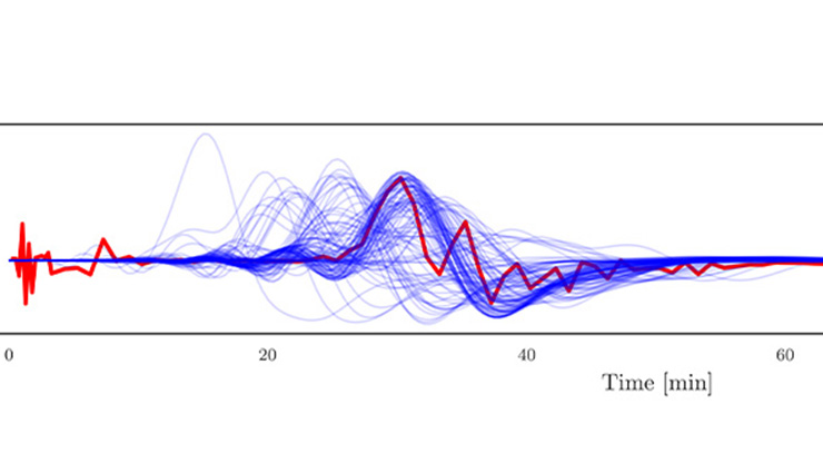
![<strong>Figure 4.</strong> Prediction of the force curve in the region of pothole 1 for a new vehicle. The prediction utilizes the complete posterior distribution as well as 65 computer model runs for the new vehicle (yellow curves). The red curves represent the test runs of the new vehicle, which were revealed after the fact, and the blue lines give the uncertainty quantification (UQ) predicted force curve and 90 percent confidence bands. The UQ predictions exhibit considerable improvement over the computer model predictions alone. Figure courtesy of [2].](/media/p2whsbuc/figure4.jpg)
Even when the model inputs are of relatively low dimension, it is difficult to assess prior distributions for the unknowns. When a model has thousands of unknowns with complex interdependencies (e.g., values of \(\mathbf{v}\) that lie on lower dimensional manifolds or fractal sets [8]), it becomes extremely challenging to specify the prior (assuming that one exists).
Challenge 5: Extrapolation
Even when one can implement statistical formalism, the goal is typically to extrapolate beyond the range of the observed data. Every weather forecast is an extrapolation into the future that is conditioned on the belief that today’s physical theory will continue to apply tomorrow. Ultimately, however, only out-of-sample performance can identify the UQ approaches that are (or would have been) most helpful.
When it comes to climate modeling, different models do not agree on the current climate—they actually yield vastly different quantitative representations due to systematic errors in each model—but they do roughly agree on changes in large-scale aspects of the climate. Each model is quantitatively flawed, yet every Earth-like model qualitatively warms under the observed changes in conditions. Can UQ help scientists interpret their similar extrapolations of future changes?
Summary and Conclusions
To conclude, we emphasize the following aspects of UQ:
- UQ is a critical component of both statistical and simulation modeling.
- The notion of model inadequacy/discrepancy (i.e., recognizing that the model is wrong) in simulation modeling is a significant advancement.
- When the Bayesian formalism of UQ is implementable, no other formalism is better.
- In practice, calculated probabilities often lack the full formalism (e.g., they might not consider model discrepancy/inadequacy). When this is the case, they are not the desired decision-relevant probabilities. Generalizations—such as the use of credal sets or the quantification of the evolving probability of a big surprise—can significantly extend the operational relevance of Bayesian UQ.
- UQ should incorporate uncertainty guidance and communicate the limitations of every stated probability.
This article is a highly abridged version of our 2019 paper [2].
References
[1] Bayarri, M.J., Walsh, D., Berger, J.O., Cafeo, J., Garcia-Donato, G., Liu, F., … Sacks, J. (2007). Computer model validation with functional output. Ann. Stat., 35(5), 1874-1906.
[2] Berger, J.O., & Smith, L.A. (2019). On the statistical formalism of uncertainty quantification. Annu. Rev. Stat. Appl., 6(1), 433-460.
[3] Bröcker, J., & Smith, L.A. (2008). From ensemble forecasts to predictive distribution functions. Tellus A: Dyn. Meteorol. Oceanogr., 60(4), 663-678.
[4] Du, H., & Smith, L. (2017). Multi-model cross-pollination in time. Physica D: Nonlinear Phenom., 353-354, 31-38.
[5] Gramacy, R.B. (2020). Surrogates: Gaussian process modeling, design, and optimization for the applied sciences. Boca Raton, FL: CRC press.
[6] Gu, M., Wang, X., & Berger, J.O. (2018). Robust Gaussian stochastic process emulation. Ann. Stat., 46(6A), 3038-3066.
[7] Judd, K., Reynolds, C.A., Rosmond, T.E., & Smith, L.A. (2008). The geometry of model error. J. Atmos. Sci., 65(6), 1749-1772.
[8] Judd, K., & Smith, L.A. (2004). Indistinguishable states II: The imperfect model scenario. Physica D: Nonlinear Phenom., 196(3-4), 224-242.
[9] Kennedy, M.C., & O’Hagan, A. (2001). Bayesian calibration of computer models. J. Royal Stat. Soc. B, 63(3), 425-464.
[10] Smith, L.A. (2002). What might we learn from climate forecasts? Proc. Natl. Acad. Sci., 99(3, Suppl_1), 2487-2492.
[11] Smith, R.C. (2013). Uncertainty quantification: Theory, implementation, and applications. In Computational science and engineering (Vol. 12). Philadelphia, PA: Society for Industrial and Applied Mathematics.
[12] Solomon, S., Qin, D., Manning, M., Marquis, M., Averyt, K., Tignor, M.M.B., … Chen, Z. (2007). Contribution of Working Group I to the Fourth Assessment Report of the Intergovernmental Panel on Climate Change (Climate Change 2007: The Physical Science Basis). New York, NY: Cambridge University Press.
About the Authors
James O. Berger
Professor emeritus, Duke University
James O. Berger is the Arts and Sciences Distinguished Professor Emeritus of Statistics at Duke University. He is widely recognized for foundational contributions to Bayesian statistics, decision theory, and model uncertainty. He was the founding director of the Statistical and Applied Mathematical Sciences Institute from 2002 to 2010, helping to establish it as a national center for interdisciplinary research. Berger is a member of the National Academy of Sciences and a fellow of the American Academy of Arts and Sciences. He received his Ph.D. in mathematics from Cornell University.

Leonard A. Smith
Professor, Virginia Tech
Leonard A. Smith is a professor in the Bradley Department of Electrical and Computer Engineering at Virginia Tech and a fellow of the London Mathematical Laboratory. He was a Senior Research Fellow in mathematics at Pembroke College within the University of Oxford from 1992 to 2020. As a professor of statistics at the London School of Economics, he served as director of the Centre for the Analysis of Time Series from 2001 to 2020. Smith's research focuses on nonlinear dynamical systems, particularly embracing structural model error, the application of imperfect models to real-world decision-making, and the feasibility of apophatic science. He earned his Ph.D. in physics from Columbia University.
Related Reading


Stay Up-to-Date with Email Alerts
Sign up for our monthly newsletter and emails about other topics of your choosing.
