Understanding Flood Flow Physics Via Data-informed Learning

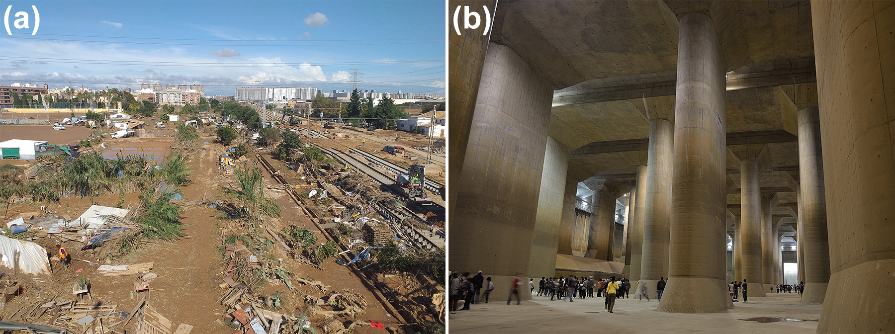
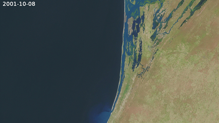
The difference between a surprising weather event and a natural disaster often boils down to one simple question: How prepared were we for the unexpected? The degree to which dangerous weather becomes a humanitarian crisis is a function of our ability to accurately predict seemingly improbable occurrences. Unfortunately, our predictive performance of flash floods has not been favorable, as these floods are the leading cause of storm-related fatalities in the U.S. The increased incidence of floods in historically low-risk areas underscores the need for preventative measures (see Figure 1), but the highly nonlinear nature of fast-moving water makes such events difficult to simulate and predict. This problem is exacerbated by the ephemeral nature of such phenomena, which means that data is seldom available for the development of predictive models. Flash flood models must therefore integrate real-world data in a flexible way that allows researchers to control the models’ prioritization of alignment with sensor data versus governing physical equations.

Recent machine learning research has inspired new methods that use data to inform—or sometimes supplant [5]—traditional complex dynamical systems models that conform to well-known partial differential equations (PDEs). With the ultimate goal of predicting flood formulation and progression based on precipitation data and topographical terrain, we utilized a physics-informed neural network (PINN) [6] to learn the solution of a simplified flood model by penalizing the network for failing to conform to incompressible flow equations. We validated this model against data from strategically placed pressure gauges in areas that previously suffered damage during flash floods. Because gauge deployment and monitoring incur significant costs in most locations, our digital twin infers missing data to act as a set of virtual gauges and ultimately support flood prediction and response efforts.

The Shallow Water Model

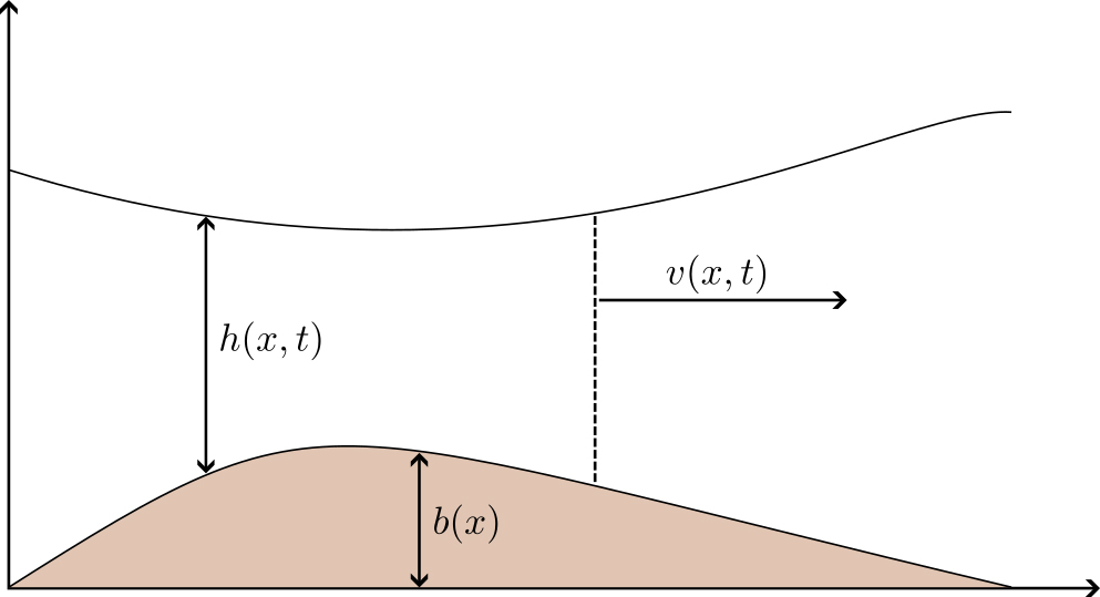
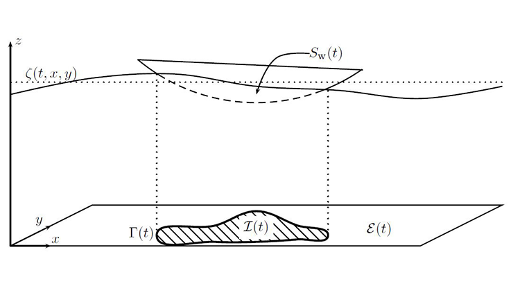
To start, we captured the fluid height \(h\) and average fluid velocity \(v\) in the steady state solution to the shallow water equations (SWE). These equations are often used to analyze river flow and tsunami propagation; while they are well understood analytically, numerically modeling them is nontrivial (see Figure 2) [7].

For a given bathymetry \(b=b(x)\), the SWE read

\[\begin{align}
           h_t + (h v)_x &= R - I & \textrm{(mass)} \\
           (h v)_t + \left[ hv^2 + \frac{1}{2} g h^2 \right]_x &= -gh(b_{x} + S_{f}) + \mu (hv_x)_x & \textrm{(momentum).}
  \end{align}\]

Here, \(S_f\) represents frictional forces at the bottom topography, \(\mu\) is the viscosity, \(R\) signifies rainfall, and \(I\) denotes soil infiltration. In the steady state regime, \(q_0\) is the steady state flow and the SWE system reduces to

\[ \begin{align}
      hv  &= (R - I)x + q_0 \\
      b_x &= -\frac{1}{gh} \left[ hv^2 + \frac 12 gh^2 \right]_x - S_f 
           + \frac{\mu}{gh} \left(h v_x \right)_x.
  \end{align}\]

We modeled the true observables of the system \(U(x,t)\) via a feed-forward neural network, which we denote with vector \(\mathcal{N}\):

\[\mathcal{N}(x, t) = \left( {\begin{array}{c}{{\mathcal{N}_h}}\\{{\mathcal{N}_v}}\end{array}} \right) \approx \left( {\begin{array}{c}{{h}}\\{{v}}\end{array}} \right) =: U(x, t).\]

Here, \(h\) represents water height and \(v\) indicates velocity. We embedded the physics of shallow water flow in the PDE residual, where \(\mathcal{L}\) is the differential SWE operator (such that for the true solution \(U\), we have \(\mathcal{L}(U) = 0\)):

\[R_{\textrm{phys}}(x, t) = \mathcal{L} (\mathcal{N})(x, t).\]

To integrate \(n\) sensor data measurements for \(h\) and \(v\) (measured at location \(x_k\) and time \(t_k\)) into our model, we introduced the following data residual:

\[R_{\textrm{data}} = \sum\limits_{k=1}^n \mathcal{N}(x_k, t_k) - U^*_k.\]

Our search for the best approximation to the true solution \(U(x,t)\) then became a nonlinear unconstrained minimization problem

\[\min_{\mathcal{N}} {\lambda_{d} \lVert R_{\textrm{data}} \rVert + \lambda_{p} \lVert R_{\textrm{phys}} \rVert},\]

where \(\lambda_{d}\) and \(\lambda_{p}\) are hyperparameters that control the model’s adherence to the provided data versus the governing PDE.

Subcritical Flow

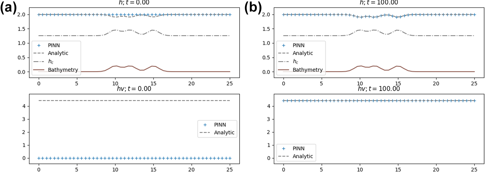
Our study specifically considered the subcritical fluid flow regime—where the flow velocity is less than the wave speed of the flow—with no rainfall, viscosity, friction, or soil penetration (\(R = \mu = S_f = I = 0\)). Given a fixed inflow and outflow boundary height to represent the known upstream flow and drainage geometry, our PINN used the Adam optimizer [2] to identify a steady state solution at \(t = 100\) seconds after 50,000 iterations (see Figure 3).

Finding a specific SWE solution when all parameters are known is not particularly illuminating — in fact, many efficient solvers already do this quite well. It would be more useful to create a model that examines the relationships between input functions (e.g., initial conditions or other physical parameters) and the system’s behavior over time. Fortunately, deep operator networks (DeepONets) can learn mappings between entire function spaces to accomplish this task (see Figure 4) [3]. In order to explore this idea in the context of flood modeling, we applied DeepONets to the one-dimensional SWE to directly learn a solution operator \(G(b)\) between the bathymetry \(b(x)\) of a riverbed (i.e., its shape) and the steady state water height \(h_{\infty}(x)\). Doing so allows us to predict the long-term behavior of river systems over various geographies.

To generate a sufficient variation of bathymetry in the training data, we used DeepXDE [4] to train our DeepONet over 3,000 bathymetry functions from a Gaussian random field. After 50,000 iterations, we observed excellent agreement between the DeepONet’s predictions and true steady state solutions to the SWE (see Figure 5).

Conclusions and Future Directions

Moving forward, we plan to relax the shallow water flow assumption and extend our model to two-dimensional incompressible flow in order to account for more violent flood behavior (e.g., dam breaks, rainfall, etc.) based on real-world data from our experimental testbed. By comparing this data to each model’s predictions, we can directly explore the introduction of error due to simplifying assumptions and determine whether these assumptions actually yield feasible flash flood models. Since PINNs can integrate the data directly into the physical model, we hope that this flexibility will allow us to capture the less tractable (e.g., more violent) aspects of flash flood dynamics and only rely on classical solvers for well-understood flood regimes. And because DeepONets are comprised of PINNs, the knowledge that we gain from progressively relaxing our simplifying assumptions will directly inform our DeepONet architecture. Progress on these fronts could provide insight into the following three critical aspects of emergency response:

• Mitigation: By directly mapping environmental conditions to flood evolution, DeepONets can help us understand the performance of various flood mitigation strategies under different conditions (e.g., intense rainfall, hydrophobic soil, etc.).
• Preparedness: Once a flood warning is issued, DeepONets can quickly simulate many possible flood evolution scenarios. By integrating a Monte Carlo approach into this process, we could also preemptively identify the regions that are most susceptible to damage and prioritize emergency response efforts accordingly.
• Response and Recovery: The integration of real-time sensor data into a PINN model that is trained over a specific location can provide emergency response teams with tools to understand the evolution of an ongoing flood based on direct field measurements. In particular, we want to use these models to identify especially dangerous flood regions when ground visibility is low or nonexistent.

Continuous advancements in data science have inspired the development of new capabilities that can ultimately mitigate the humanitarian impact of floods. Every minute counts during an emergency, and even marginal improvements in flood modeling can buy precious time for response teams and downstream communities as they prepare for the worst.

Jonathan Thompson delivered a contributed presentation on this research at the 10th International Congress on Industrial and Applied Mathematics (ICIAM 2023), which took place in Tokyo, Japan, in August 2023. He received funding to attend ICIAM 2023 through a SIAM Travel Award that was supported by U.S. National Science Foundation grant DMS-2233032. To learn more about SIAM Travel Awards and submit an application, visit the online page. 

Acknowledgments: This material is based on work that is supported by the U.S. National Science Foundation (NSF) Graduate Research Fellowship under grant no. 2041854 and the Colorado Department of Transportation under Research ID R223.05. In addition to support from SIAM and NSF grant DMS-2233032, registration and travel support for ICIAM 2023 was provided by the Department of Mathematics at the University of Colorado Colorado Springs (UCCS). This work used the INCLINE high-performance computing cluster at UCCS, which is supported by NSF grant no. 2017917.

References
[1] Fasshauer, G., & McCourt, M. (2015). Kernel-based approximation methods using MATLAB. In Interdisciplinary mathematical sciences (Vol. 19). Singapore: World Scientific Publishing.
[2] Kingma, D.P., & Ba, J. (2014). Adam: A method for stochastic optimization. Preprint, arXiv:1412.6980.
[3] Lu, L., Jin, P., Pang, G., Zhang, Z., & Karniadakis, G.E. (2021). Learning nonlinear operators via DeepONet based on the universal approximation theorem of operators. Nat. Mach. Intell., 3(3), 218-229.
[4] Lu, L., Meng, X., Mao, Z., & Karniadakis, G.E. (2021). DeepXDE: A deep learning library for solving differential equations. SIAM Rev., 63(1), 208-228.
[5] Price, I., Sanchez-Gonzalez, A., Alet, F., Andersson, T.R., El-Kadi, A., Masters, D., … Willson, M. (2025). Probabilistic weather forecasting with machine learning. Nature, 637(8044), 84-90.
[6] Raissi, M., Perdikaris, P., & Karniadakis, G.E. (2019). Physics-informed neural networks: A deep learning framework for solving forward and inverse problems involving nonlinear partial differential equations. J. Comput. Phys., 378, 686-707.
[7] Whitham, G.B. (1999). Linear and nonlinear waves. In Pure and applied mathematics. New York, NY: John Wiley & Sons.