Unlimited Sensing: When Noise Becomes the Signal

Although the digital revolution has transformed human lives, it rests on an inconvenient truth: every digital measurement begins with loss. When capturing the faint echo of a sound, the subtle shade of a color, or a fragile biomedical signal, converting the continuous world into a digital format inevitably discards something. This is not a defect, but rather an inherent consequence of digitization.

Digitization involves sampling in time and quantization in amplitude. As Claude Shannon taught us, sampling can be lossless under appropriate bandwidth assumptions and rates [9]. But quantization is different, as rounding a continuum to a finite set of levels is irreversible and introduces round-off error (often called quantization noise) [6]. This type of loss is treated as a necessary evil of digitization.

For decades, engineers have accepted a hard limit: analog-to-digital converters (ADCs) can never escape a triad of constraints. Like the Greek Moirai (the sisters of Fate) who spin, measure, and cut the thread of life, ADCs are bound by their own triad: dynamic range (DR), digital resolution (DRes), and power consumption (bit budget). Favor one, and the others bend or break. Widening the recordable DR to avoid saturation coarsens your quantization steps (DRes), while tightening the steps for finer detail invites clipping. Meanwhile, each extra bit (digital currency) of precision tends to drive exponential costs in power [7 ] and analog complexity, whereas an increase to the sampling rate grows power in a roughly linear manner. This DR-DRes-power tradeoff has long shaped ADC design and inspired different strategies for improved converters [4].

This situation raises a natural question: Can the tradeoff be broken or approached differently? The unlimited sensing framework (USF) offers an alternative interpretation of what is traditionally called “noise” [3]. Instead of discarding quantization noise as error, the USF treats it as a digital signal — structured information from which we can recover the original signal. The key mathematical insight is that for smooth signals, the discarded component can still carry recoverable information.

From Digitization’s Two Steps to a New Playbook

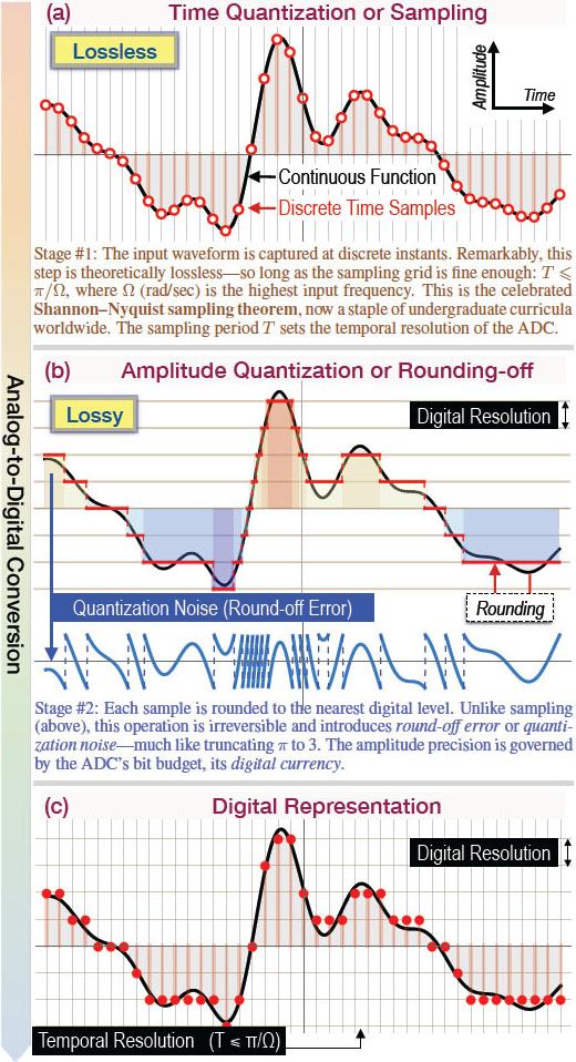
At its core, existing digital acquisition has two stages (see Figure 1):

1. Sampling, or time quantization (see Figure 1a), which takes values of a continuous-time function on a temporal grid. Under the Shannon- Nyquist conditions, this step is theoretically reversible.
2. Amplitude quantization, or round-off (see Figure 1b), which maps amplitudes to a finite set of levels (i.e., rounding \(\pi\) to \(3\)). This step is irreversible and introduces quantization noise.

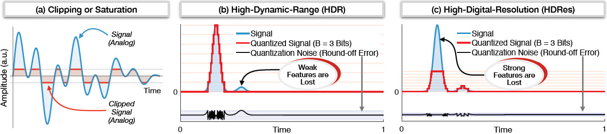
Conventional ADCs clip whenever inputs exceed the recordable voltage range (see Figure 2a). To avoid clipping, we can widen the range at the cost of quantization step size (see Figure 2b). Conversely, we can tighten the steps to capture subtle variations — at the risk of clipping strong features (see Figure 2c). The result is a familiar dilemma: high-dynamic-range (HDR) capture tends to erase weak features, while high-digital-resolution capture tends to cut off strong features. With a fixed bit budget, trading one for the other is unavoidable. The USF replaces this zero-sum mindset with a design that folds rather than clips.

Folding Instead of Clipping

The modulo ADC (MADC) realizes the USF in practice by applying a nonlinearity to the input before conventional quantization [2] (see Figure 3a). If \(g(t)\) is the input, the MADC produces a continuous version of quantization noise:

\[y(t) = {\mathscr{M}_{\lambda}}(g(t))\in[-\lambda, \lambda], \qquad \lambda>0,\]

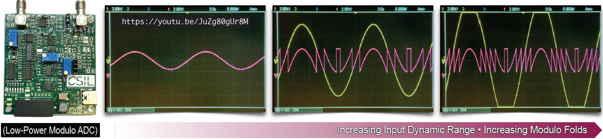
where \(\mathscr{M}_\lambda \, :\, g \mapsto 2\lambda \; ({[\![} \frac{g}{2\lambda} + \frac{1}{2} {]\!]} - \frac{1}{2}),\) and \([\![g]\!]\) is the fractional part of \(g.\) In effect, \(g\gg\lambda\) is wrapped back into a bounded interval — much like coiling long spaghetti onto a fork. As the input amplitude grows, the output on an oscilloscope remains bounded by repeated folds (see Figure 3b and Animation 1 ). Each additional fold corresponds to an unknown integer multiple of \(2\lambda;\) \(y\) thus encodes the signal modulo to a threshold \(\lambda.\) More information about modulo folding and related topics is available in the literature [3]. 

This design choice triggers two immediate consequences:

1. Elimination of clipping: Because the map keeps \(y(t)\) bounded in \([-\lambda, \lambda],\) the hardware no longer saturates (see Figure 3b). The “information” that would have been lost at the rails is preserved in the pattern of folds.
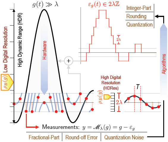
2. Breaking the DR-DRes tradeoff: Let \(\textrm{DR}(g)=\max g-\min g\) and \(\textrm{DR}(y) = 2\lambda.\) With a \(B\)-bit quantizer, a conventional pipeline yields \(\rho_{B}(g)=\textrm{DR}(g)/2^B, \) whereas folded capture yields \(\rho_{B}(y)=2\lambda/2^B. \) Clearly, \(\rho_{B}(g)>\rho_{B}(y)\) (see Figure 4). Since \(\textrm{DR}(y)\) is fixed by design, resolution decouples from the input DR; we can retain fine digital resolution even when \(g\gg\lambda.\) Signals that would otherwise be buried below quantization steps become detectable in the USF (see Figure 5c), thus enabling new applications.

Intuitively, folding saves bits by transferring effort from the hardware to mathematical algorithms that unfold the signal at a later time.

A Shannon-like Promise Without Clipping 

After folding, the signal is sampled: \(y[k]=\mathscr{M}_{\lambda}(g(kT)),\) \(k\in\mathbb{Z}\) (see Figure 4). Although the modulo map injects high frequencies into \(y,\) the following theorem applies [3]: If a function \(g(t)\) contains no frequencies above \(\Omega\) (radians/second), it is completely determined by its modulo samples that are spaced \(T=1/2{\Omega}e\) seconds apart, where \(e \approx 2.71828\) (up to an unknown constant). With additional information, \(T<\pi/\Omega\) is sufficient [8].

Notably, this Shannon-like guarantee does not depend on the folding threshold \(\lambda.\) In theory, this opens the door to unlimited DR. A similar theorem applies to quantized measurements.

The philosophical shift is notable, in that the modulo output is a nonlinear transform that converts input into continuous quantization noise. Rather than avoiding nonlinearity as an adversary, the USF uses it as a design tool. Controlled redundancy in measurements helps to “invert” the nonlinearity.

How Recovery Works

A clean way to think about the modulo output and recovery is via

\[y = \mathscr{M}_\lambda (g) \equiv g - \varepsilon_g, \quad \varepsilon_g \in 2\lambda\mathbb{Z}.\]

Here, \(\varepsilon_g\) is the unknown “integer” (fold) component — what traditional pipelines would regard as the digital signal (see Figure 4). In the USF, mathematical algorithms estimate piecewise constant \(\varepsilon_g\) from the measured \(y\) and add it back to unfold the samples. 

Two complementary recovery viewpoints can provide assistance:

1. Time domain: For smooth \(g,\) higher-order differences \(\Delta^N g\) are small when the sampling period \(T\) is sufficiently fine relative to the bandwidth or smoothness. Meanwhile, \(\Delta^N\varepsilon_g\) lives on the lattice \(2\lambda\mathbb{Z}\) and is annihilated by \(\mathscr{M}_\lambda(\cdot).\) This outcome yields a relation of the form \(\Delta^N g = \mathscr{M}_\lambda(\Delta^N y),\) from which we can recover \(\Delta^N\varepsilon_g,\) — the differences of the integer part. It then integrates (with suitable constants) to reconstruct \(\tilde{\varepsilon}_g,\), which results in \(\tilde{g}=y+\tilde{\varepsilon}_g. \) The key idea is that differences suppress smooth trends but reveal the folds in a controlled way [3]. Figure 5 depicts reconstruction with \(N = 4\) and hardware data; the corresponding code and data are available online. 
2. Frequency domain: The differences in the fold sequence \(\Delta\varepsilon_g\) are impulses in time and exponentials in frequency. We can use spectral line-fitting (Prony-type methods) to estimate the unknown fold locations and magnitudes, then reconstruct \(g\) via familiar interpolation. This path utilizes a Fourier-domain approach to recover \(\varepsilon_g\) [2].

These techniques extend beyond strictly bandlimited signals to additional smooth classes (e.g., polynomials and splines), which increases their utility in imaging and other inverse problems.

Implications: Three Perspectives

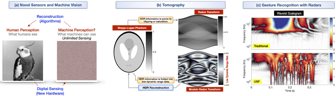
From “Capture First” to “Co-design Always”: Traditional sensing pipelines capture with hardware and clean up with algorithms. In this hierarchy, no algorithm—however clever—can recover what the hardware never recorded. The USF breaks the hierarchy through hardware/software co-design, which deliberately modifies the forward model to enrich digitization. When combined with redundancy, controlled nonlinearity—such as folding, aliasing, and wrapping—turns an ill-posed problem into a well-conditioned one by shifting the burden of complex hardware to advanced algorithms. Doing so leads to new forms of sensing and imaging that inspire new inverse problems [1, 5] (see Figure 6a).

Rethinking Digitization for Machines: Conventional digitization optimizes for human perception, yielding round numbers, uniform brightness, and smooth tonal gradients. But in today’s world, machines—not humans—interpret most of our data, and standard conventions may not be optimal for such interpretation. A computer does not need a perfectly linear representation; in fact, folded or irregular encodings—like those produced by the USF—can be more efficient for inference, compression, or learning. In classification tasks, during which algorithms rely on subtle statistical features, modulo-based representations can preserve fine variations without inflating bit budgets, ultimately improving accuracy under resource constraints (see Figure 6c and Animation 2 ). By prioritizing algorithmic utility over human readability, the USF points toward machine-native digitization: data designed for understanding rather than display. 

From Nonlinear Algorithms to Nonlinear Acquisition: In recent decades, signal processing and inverse problems have moved toward nonlinear methods like sparsity, thresholding and pursuit, variational regularization, and deep learning. Nevertheless, acquisition has largely remained linear (e.g., compressed sensing uses linear measurements with nonlinear recovery). The USF addresses this gap by introducing deliberate nonlinearity at capture, which results in both a conceptual unification of hardware and algorithms and concrete computational and energy advantages.

Practical Outlook: What Changes in the Lab?

On the hardware side, the modulo stage is simple and power-lean; it can seamlessly precede conventional quantization. Because the output is bounded, we can reduce headroom and avoid saturation without resorting to large bit budgets — enabling, for example, low-resolution (few-bit) digitization with competitive performance.

On the algorithm side, recovery runs as standard numerical techniques: difference operators, lattice arithmetic, spectral estimation, interpolation, and sparse optimization. The guarantees are rooted in familiar smoothness/bandwidth assumptions and translate to other structured signal classes, such as sparse signals. In practice, this means that one sensor can capture signals that are both very strong and very weak at the same time and with modest power budgets.

Applications span any setting where digital sensing is the starting point — from cameras and medical scanners to radar, Internet of Things devices, and machine learning pipelines. In HDR imaging, for example, folding can preserve bright highlights without sacrificing shadow detail (see Figure 6a). Similarly, in tomographic reconstruction, signals often exhibit extreme variations in intensity across different tissue types or materials (see Figure 6b).

A Broader Perspective on Digital Representation

Across mathematics and computing, we routinely split a quantity into two parts: integer versus fractional (number theory), rounding versus round-off error (numerical analysis), and quantized value versus quantization noise (signal processing and ADCs). Standard digitization keeps the first part and discards the second. The USF questions this conventional separation. For smooth signals, we can often reconstruct the whole from the “discarded” part if the system is designed to make that part informative.

In light of this information, the word “unlimited” does not mean “infinite.” Rather, it means unbounded by convention. By folding signals instead of clipping them, treating error as data, and merging mathematics with hardware, the USF shifts the goal from minimizing error to harnessing it. Limits that we traditionally treat as fixed can instead be viewed as design parameters.

Acknowledgments: This work was supported by the European Research Council Starting Grant CoSI-Fold — Making the Invisible Visible: Computational Sensing and Imaging via Folding Non-Linearities. (Grant No. 101166158) and the UK Research and Innovation (UKRI) Future Leaders Fellowship Sensing Beyond Barriers via Non‑Linearities: Theory, Algorithms, and Applications. The author thanks Robert Gray for valuable comments and historical perspectives. Appreciation is also extended to Ruiming Guo and Vaclav Pavlicek of the Computational Sensing & Imaging Lab (CSIL) for their feedback on earlier drafts. Lastly, the author expresses gratitude to Lina Sorg for continuous encouragement and patience, without which this article would not have been possible. Further details on Unlimited Sensing, along with reproducible research materials, are available here. 

References   
[1] Azar, E., Mulleti, S., & Eldar, Y.C. (2025). Unlimited sampling beyond modulo. Appl. Comput. Harmon. Anal., 74, 101715.
[2] Bhandari, A., Krahmer, F., & Poskitt, T. (2021). Unlimited sampling from theory to practice: Fourier-Prony recovery and prototype ADC. IEEE Trans. Signal Process., 70, 1131-1141.
[3] Bhandari, A., Krahmer, F., & Raskar, R. (2020). On unlimited sampling and reconstruction. IEEE Trans. Signal Process., 69, 3827-3839.
[4] Daubechies, I., & DeVore, R. (2003). Approximating a bandlimited function using very coarsely quantized data: A family of stable sigma-delta modulators of arbitrary order. Ann. Math., 158(2), 679-710.
[5] Eamaz, A., Mishra, K.V., Yeganegi, F., & Soltanalian, M. (2024). UNO: Unlimited sampling meets one-bit quantization. IEEE Trans. Signal Process., 72, 997-1014.
[6] Gray, R.M., & Neuhoff, D.L. (1998). Quantization. IEEE Trans. Inf. Theory, 44(6), 2325-2383.
[7] Murmann, B. (2015). The race for the extra decibel: A brief review of current ADC performance trajectories. IEEE Solid-State Circuits Mag., 7(3), 58-66.
[8] Romanov, E., & Ordentlich, O. (2019). Above the Nyquist rate, modulo folding does not hurt. IEEE Signal Process. Lett., 26(8), 1167-1171.
[9] Shannon, C.E. (1949). Communication in the presence of noise. Proc. IRE, 37(1), 10-21.