Generalized Modeling Reveals Stabilization in Arctic Marine Food Web Models

Marine ecosystems provide the most important natural resources for subsistence and commercial harvesting in the Arctic. However, polar amplification—when the temperature in polar regions rises more quickly than other areas during global warming—presents an existential threat to Arctic species and ecosystem stability. Mathematical models that support observational evidence are thus becoming increasingly important in our quest to understand Arctic ecosystem dynamics and conservation efforts.

Realistic food webs typically include a large number of species that interact in highly complex networks. Empirical descriptions of parameters like population size, birth and death rate, and predator-prey characteristics are naturally incomplete, and uncertainties in data can be large. There is hence a clear need for abstraction and approximation in the modeling process. Conventional dynamical systems models tend to focus on relatively few species and approximate functional forms to investigate trajectories in phase space. But as a result, most of these mathematical models produce a lower food web stability than that of real ecosystems [6-8].

Generalized modeling approaches—which provide linear stability analysis for infinitely many (conventional) ordinary differential equation (ODE) models—offer an avenue for progress that does not require precise data and narrow specification of all processes [3, 5]. Instead of identifying exact mathematical forms, these approaches group processes into unspecified general gain and loss terms that represent biomass flow into and within the network in question. A normalizing coordinate transformation maps the unknown fixed points to a known rescaled fixed point, from which local stability and bifurcation information is extracted. In short, generalized models efficiently handle and analyze the stability properties of large, complex networks.

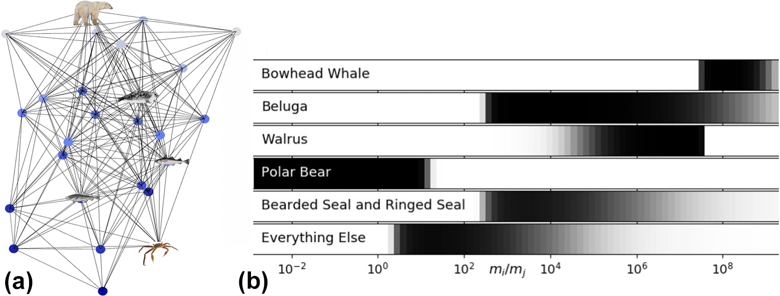
We used generalized modeling to study the stability of food web models of the southern Beaufort Sea (SBS) [2]. To begin, we sampled 30 species and trophospecies (i.e., groups of species that function similarly in food webs) from the SBS based on their high ecological significance; our selections ranged from copepods to the bowhead whale and spanned 13 orders of magnitude in body mass [2]. Body size strongly controls the probability of a predator-prey interaction between any pair of species, as predators are usually one to four orders of magnitude larger than their prey. We probabilistically constructed more than a million food webs based on body mass ratios between predator and prey (see Figure 1). The base model treats all species equally; the probability of network connections is constrained only by body size, and all other species traits are equivalent. If a fixed point in the SBS network dynamics is stable, we can consider the web to be stable as well.

Food Web Dynamics

The state \(\boldsymbol{x}\in\mathbb{R}^N\) of a predator-prey ecological network (i.e., a food web) with \(N\) species evolves with a growth rate due to production \(\mathscr{S}\) and predation \(\mathscr{F}\), and a loss rate due to predation \(\mathscr{L}\) and other mortality \(\mathscr{M}\). The biomass \(x_i\) of species \(i\) is then given by

\[\dot{x}_{i}(t)=\mathscr{S}_{i}(x_{i}) +\ \mathscr{F}_{i}(T_i,x_i)\ -\ \mathscr{M}_{i}(x_i)\ -\ \sum_j \mathscr{L}_{ij}(\boldsymbol{x}), \tag1\]

where \(T_i\) is the total prey that predator \(i\) consumes. The predatory loss \(\mathscr{L}_{ij}\) of prey \(i\) from predator \(j\) is proportional to the predatory growth of predator \(\mathscr{F}_j\) and the fraction that prey \(i\) contributes to the resources of predator \(j\).

Generalized Food Web

Generalized modeling [2-4] normalizes the state to an unknown, nontrivial fixed point \(\chi_i=x_i/x^*_i\), and normalizes each unspecified growth or loss process of the form \(\mathscr{G}\) in \((1)\) to its value at the fixed point: \(g(\boldsymbol{\chi})=\mathscr{G}(\mathbb{X}^*\boldsymbol{\chi})/\mathscr{G}(\boldsymbol{x}^*)\). This normalization maps the unknown fixed point \(x_i^*\) to a known fixed point \(\chi_i^*=1\); it also maps the unknown process to a known process value at the fixed point \(g(\boldsymbol{\chi}^*) = 1\) in the rescaled system:

\[\dot{\chi}_i = \alpha_i\big(\sigma_i s_i(\chi_i)+\phi_i f_i(t_i,\chi_i)-\mu_i m_i(\chi_i) -\lambda_i\sum_j l_{ij}(\boldsymbol{\chi}) \big). \tag2\]

Here, \(s_i\), \(f_i\), \(m_i\), and \(l_{ij}\) represent the rescaled processes (equal to \(1\) at steady state), and \(\alpha_i\) is a time scale parameter. The primary scale parameters \(\sigma_i, \phi_i\) and \(\mu_i, \lambda_i\) respectively describe the relative weighting of the growth and loss processes at steady state. Secondary scale parameters, which are included in the loss term \(l_{ij}\), describe the relative weighting of predatory inflow or outflow at a network node in steady state.

Fixed Point Stability

The local dynamics near the fixed point are determined by the derivatives of the rescaled processes in steady state: \(g^{(\chi_i)}\equiv\frac{\partial g(\boldsymbol{\chi})}{\partial \chi_i}\bigg|_{\boldsymbol{\chi}^*}\). These derivatives (i.e., nonlinearity parameters) describe the nonlinearity of process \(\mathscr{G}(\boldsymbol{x})\), while nonlinearity parameters \(s_i^{(\chi_i)}, m_i^{(\chi_i)}, \ldots\) are remnants of the unspecified functions \(\mathscr{S},\mathscr{M}, \ldots\) from \((1)\) in the Jacobian. In generalized modeling, one can vary these nonlinearity parameters to simultaneously represent different specific functions. For example, mortality processes \(\mathscr{M}\) are often modeled as a power law, and the resulting nonlinearity parameter \(m_i^{(\chi_i)}\) is the exponent of that law. The logistic growth model is often used to approximate the production process \(\mathscr{S}\), but many homologous functional forms follow the same nonlinearity range [1].

Because production grows linearly in small populations, the nonlinearity of production \(s_i^{(\chi_i)}\) is \(1\); in larger populations, intraspecific competition reduces the nonlinearity parameter. We chose a nonlinearity of production within the range \(s_i^{(\chi_i)}\in[-1,1]\) to exclude populations that are close to their carrying capacity.

Steady state stability depends on the time scale parameter, scaling parameters, nonlinearity parameters, and web topology. Assumptions about body size distribution, proportion of biomass flows, nonlinearities of growth and loss processes, and predatory links between species determine these generalized parameters without the need to specify initial conditions or particular functional forms.

Refining Species Characteristics

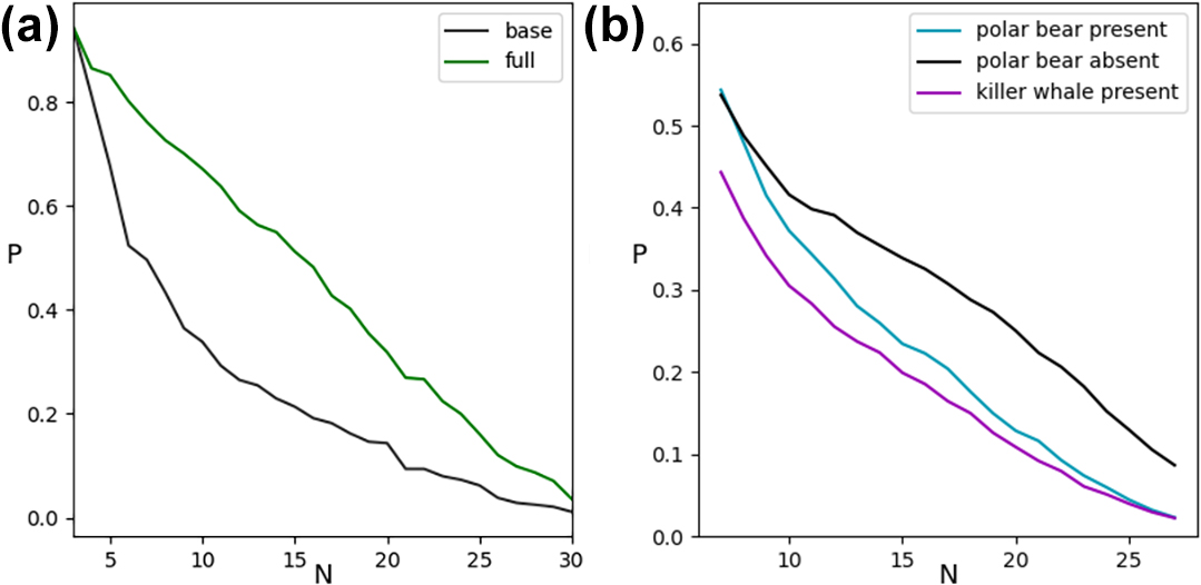
Our results show that food web stability increases as model food webs become more realistic. For example, the model improves when we add specialized foraging behavior (see Figure 1b); account for filter feeders (e.g., bowhead whales) and gape-limited species (e.g., walruses, beluga whales, and seals), whose prey are smaller than body size ratios would predict; and account for superpredators (e.g., polar bears) that consume much larger prey than body size ratios would predict. The full model also includes prey preference in the form of inhomogeneous predator-prey weights and habitat constraints that only allow the formation of predator-prey links when species share a common habitat. Ultimately, food web stability increases by 82 percent in the full model versus the base model (see Figure 2a).

Ecosystem Restructuring and Global Warming

Rapid sea ice decline in a warming Arctic threatens critical habitats for many sympagic species, and the incursion of new temperate species in Arctic ecosystems is restructuring food webs. Figure 2b reveals that the lack of a fierce top predator—via the extirpation of the ice-obligate polar bear or the absence of the “invasive” killer whale, for instance—significantly increases the proportion of stable webs. Although apex predators are generally thought to enhance biodiversity, we found that they may have a destabilizing impact on fixed points. The absence of a superpredator typically generates more diversity in top predators, which has a possibly stabilizing effect [2].

Background Noise and Stability

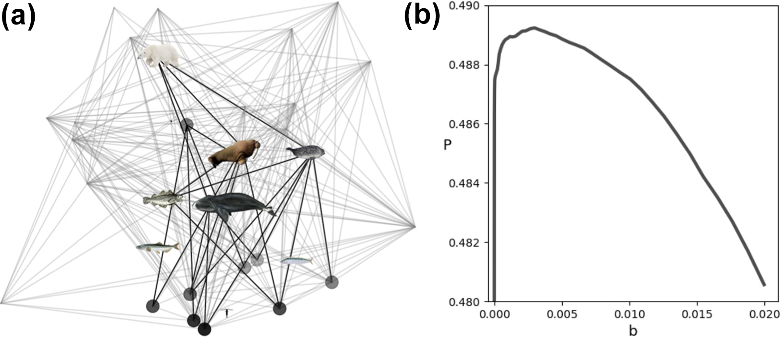
Even depauperate Arctic ecosystems like the SBS food web are composed of thousands of identifiable species. Dynamical models typically focus on abundant species and/or species that are of particular management interest, neglecting minor species that contribute minimally to the total biomass. In Figure 3a, we modify the network of main species to include minor (background) links. Each background link has a small weight, called background pressure \(b\), for predatory inflow and outflow. Figure 3b illustrates the collective stabilizing impact of latent, minor ecosystem members; food web stability is greatest for a relatively small optimum background pressure.

Conclusions and Future Directions

Our study demonstrates that species characteristics—including unique species-specific foraging traits, habitat constraints, background noise from minor ecosystem members, and the absence of fierce predators—impart stability in ecological network models. Future research will explore whether such realistic refinements can explain models’ typical lack of stability when compared to observations [6-8].

The role of species that contribute little to the total biomass remains rather unexplored, but it might be an important aspect of ecosystem stability. We have much to learn about noise-induced stabilization in network dynamics, particularly in regard to topological features or noise patterns that might make or break the stabilization.

Although generalized modeling does not assume explicit functional forms or initial conditions, it still efficiently captures the stability of nontrivial steady states for an infinite number of (conventional) ODE models [3, 4]. However, ODE models can provide information about trajectories, coexistence of fixed points, and more complex attractors that generalized models cannot. As of yet, little progress has been made to combine both approaches [1].

Renate Wackerbauer delivered a contributed presentation on this research at the 2023 SIAM Conference on Applications of Dynamical Systems, which took place in Portland, Ore., in May 2023.

References
[1] Awender, S., Wackerbauer, R., & Breed, G.A. (2023). Combining generalized modeling and specific modeling in the analysis of ecological networks. Chaos, 33(3), 033130.
[2] Awender, S., Wackerbauer, R., & Breed, G.A. (2024). How realistic features affect the stability of an Arctic marine food web model. Chaos, 34(1), 013122.
[3] Gross, T., & Feudel, U. (2006). Generalized models as a universal approach to the analysis of nonlinear dynamical systems. Phys. Rev. E, 73(1), 016205.
[4] Gross, T., Rudolf, L., Levin, S.A., & Dieckmann, U. (2009). Generalized models reveal stabilizing factors in food webs. Science, 325(5941), 747-750.
[5] Kuehn, C., Siegmund, S., & Gross, T. (2013). Dynamical analysis of evolution equations in generalized models. IMA J. Appl. Math., 78(5), 1051-1077.
[6] Landi, P., Minoarivelo, H.O., Brännström, Å., Hui, C., & Dieckmann, U. (2018). Complexity and stability of ecological networks: A review of the theory. Popul. Ecol., 60(3), 319-345.
[7] May, R.M. (2001). Stability and complexity in model ecosystems. In Princeton landmarks in biology. Princeton, NJ: Princeton University Press.
[8] Polis, G.A. (1998). Stability is woven by complex webs. Nature, 395, 744-745.